Macroeconomics Summary – CORE: The Economy – ECB1MACR Period 3:
Week 1:
Introduction Unit 13: How Economies Fluctuate between Booms and Recessions as
they are Continuously Hit by Good and Bad Shocks
Economies fluctuate between booms and recessions, as they are continuously hit by good
and bad shocks.
Fluctuations in GDP affect unemployment (u).
Economic accounts fluctuations and growth. Reaction of households saving or
borrowing (limited), smoothing consumption (C) not enough to stop fluctuations.
Investments (I) are more volatile than C.
Unemployment / job loss leads to a lot more than only monetary loss compensation for
restoring wellbeing is greater than just the lost income.
In the process of drawing conclusions, we should be careful in stating that correlation
implies causation / a causal relationship between variables.
Organisation for Economic Cooperation and Development (OECD) is an international
organisation which facilitates comparable statistics on economic and social performance.
Paragraph 13.1: Growth and Fluctuations
GDP (per capita) growth has not been smooth logarithmic scale, which measures a
quantity based on the ‘log’ function, shows the ratio scale / growth rates these are
fluctuating in the long-run if data forms a straight line on a ratio scale, the growth rate is
constant.
Fluctuation a deviation from the average, long-run, growth per year.
Downturns in the business cycle (movement from boom to recession and back to boom) are
associated with higher levels of unemployment unemployment goes down in booms and
up in recessions.
Recession declining output, over once the economy starts to grow again; OR output
below normal level, even when GDP is growing.
Paragraph 13.2: Output Growth and Changes in Unemployment
Okun’s Law the relationship between output and unemployment fluctuations when
output is high, unemployment tends to decrease Okun’s coefficient is the percentage
with which unemployment changes when output increases with 1%.
Relationship summarised…
Paragraph 13.3: Measuring the Aggregate Economy
Aggregate Economy the sum of all parts of an economy brought together described
using aggregate statistics. Aggregate (total) output GDP.
GDP measures Expenditure (total spent, C + I + G + X – M), Production (total produced,
added value), Income (sum of all received incomes, wage + profit + self-employed income +
taxes).
Circular Flow Model (+ government)…
,Paragraph 13.4: Measuring the Aggregate Economy – The Components of GDP
GDP / Expenditure Y = C + I + G + X – M
Consumption C goods and services produced by households. Investments I
spending by firms on new equipment; spending on construction of new housing.
Government Spending G consumption and investment purchases by the government.
Exports X domestically produced goods / services, purchased by other countries’
households and firms and governments. Imports M goods and services purchased by
households and firms and governments in the home economy, produced in other countries.
Trade Balance (X – M) net exports, surplus when X > M, deficit when X < M.
Week 2:
Paragraph 13.5: How Households Cope with Fluctuations
GDP can be divided into components from the expenditure side, but also from the
production side.
Volatility (extreme) fluctuations in growth of components of the GDP or the GDP itself. If
a variable is more volatile than another, the growth rates change more over the years.
Shock an unexpected event which can influence growth rates it is an exogenous
change in data from a model these shocks can occur for one household or for a whole
economy.
Household Shock self-insurance (saving in good times so that the saved money can be
spend in bad times) and co-insurance (paying taxes to ‘support’ those who need benefits
when temporarily out of work, this can work both ways) Altruism, or willing to bear costs
to help or support others, can occur when co-insurance happens informally.
People prefer a smooth pattern of consumption and they are willing to support others and
themselves to smoothen good and bad times.
Economy-Wide Shock community survival requires that less badly hit households help
the worst-hit households.
Paragraph 13.6: Why is Consumption Smooth?
Households want to keep their consumption somewhat constant they save and borrow to
smoothen bumps in income some households adjust consumption ahead of time, having
planned the expected present and future income shocks to an economy will be decreased
because spending decisions are based on long-term considerations.
Limits to Smoothening lack of information; credit constraints / credit market exclusion
(not being allowed to borrow the money needed); limited co-insurance (those in need
cannot be supported by the more fortunate); weakness of will (lack of willpower not being
able to carry out plans, not saving even though it would be a good option).
In order to smoothen consumption optimally, households choose a point on the line of
choosing between present and future consumption MRS = MRT.
Being able to borrow money will make it easier for households to smooth consumption.
Due to limits to smoothing of consumption, changes in income happen at the same time as
changes in consumption.
Paragraph 13.7: Why is Investment Volatile?
Firms invest in new equipment and premises whenever they see an opportunity to make
profits investments (aggregate investment) are more volatile than consumption there
are clusters of investment projects at some times and very few projects at other times in
other words, investment waves occur through booms because when some firms invest,
others have to as well to keep up with innovations in the market and because of credit
constraints.
, Low Capacity Utilisation if there is not ‘enough’ demand, firms have no incentive to hire
more employees or to invest in new machinery little spending by firm low expected
demand low profits (self-reinforcing vicious circle).
High Capacity Utilisation if there is more demand, firms will hire more employees
demand increases profits rise (self-reinforcing virtuous circle) firms have similar beliefs
about expected future demand.
Business Confidence has a major role in fluctuations in the economy as a whole in
graphs, the business confidence indicator moves closely with AD and investment.
To achieve a Pareto-efficient Nash equilibrium, firms have to coordinate in some way or
develop business confidence moving from vicious to virtuous circle.
Consumption is less volatile than GDP. Government Spending G is less volatile than
investments. Net exports are volatile, because they change along with the whole economy.
Introduction Unit 14: How Governments can moderate Costly Fluctuations in
Employment and Income
Multiplier Process AD fluctuations affect a country’s GDP through a multiplier, the GDP
may change less or more than a component of GDP itself.
Fiscal Policy governments can use changes in taxes and spending to stabilise the
economy.
Policies can promote economic growth, reduce unemployment and avoid instability
increased roles of governments in national economies partially helped to stabilise
economies more.
Paragraph 14.1: The Transmission of Shocks – the Multiplier Process
Multiplier if the total increase in GDP is equal to the initial increase in consumption /
investment / government spending / exports, the multiplier is equal to 1.
Multiplier (2) if the total increase in GDP is greater or less than the initial increase in a
GDP component, the multiplier is greater or less than 1.
The Multiplier model depends on the state of a national economy.
Paragraph 14.2: The Multiplier Model
Aggregate Consumption autonomous consumption + income-dependent consumption
C = c0 + c1Y fixed and variable amount c1 is the Marginal Propensity to Consume
(MPC) the MPC is the slope of the Aggregate Consumption graph the more a
household is able to smoothen consumption, the lower the MPC and the flatter the graph.
Durable goods are more volatile than non-durable consumption goods, because spending
on durable goods can be postponed more easily and is more like an investment.
Aggregate Demand (AD) and Output (Y) the 45 degree line (y = x) of this graph depicts
every situation in which AD = Y Goods Market Equilibrium.
Aggregate Demand is equal to C + I c1 + c0Y + I the intersection between Y and c1 +
c0Y + I is the actual state of the economy.
Calculating the Multiplier from a Model if there is an increase or a decrease in
investment I (or consumption C), the AD line increases or decreases, leading to a new
equilibrium the actual change in output Y divided by the initial change in I or C is the
multiplier.
A fall / rise in demand leads to a fall / rise in production and an equivalent fall / rise in
income, which leads to a further fall / rise in demand which again leads to a further fall / rise
in production. The multiplier is the sum of all the successive decreases / increases in
production.
Production adjusts to demand firms supply the amount of goods demanded at a certain
price.
Paragraph 14.3: Household Target Wealth, Collateral, and Consumption Spending
Week 1:
Introduction Unit 13: How Economies Fluctuate between Booms and Recessions as
they are Continuously Hit by Good and Bad Shocks
Economies fluctuate between booms and recessions, as they are continuously hit by good
and bad shocks.
Fluctuations in GDP affect unemployment (u).
Economic accounts fluctuations and growth. Reaction of households saving or
borrowing (limited), smoothing consumption (C) not enough to stop fluctuations.
Investments (I) are more volatile than C.
Unemployment / job loss leads to a lot more than only monetary loss compensation for
restoring wellbeing is greater than just the lost income.
In the process of drawing conclusions, we should be careful in stating that correlation
implies causation / a causal relationship between variables.
Organisation for Economic Cooperation and Development (OECD) is an international
organisation which facilitates comparable statistics on economic and social performance.
Paragraph 13.1: Growth and Fluctuations
GDP (per capita) growth has not been smooth logarithmic scale, which measures a
quantity based on the ‘log’ function, shows the ratio scale / growth rates these are
fluctuating in the long-run if data forms a straight line on a ratio scale, the growth rate is
constant.
Fluctuation a deviation from the average, long-run, growth per year.
Downturns in the business cycle (movement from boom to recession and back to boom) are
associated with higher levels of unemployment unemployment goes down in booms and
up in recessions.
Recession declining output, over once the economy starts to grow again; OR output
below normal level, even when GDP is growing.
Paragraph 13.2: Output Growth and Changes in Unemployment
Okun’s Law the relationship between output and unemployment fluctuations when
output is high, unemployment tends to decrease Okun’s coefficient is the percentage
with which unemployment changes when output increases with 1%.
Relationship summarised…
Paragraph 13.3: Measuring the Aggregate Economy
Aggregate Economy the sum of all parts of an economy brought together described
using aggregate statistics. Aggregate (total) output GDP.
GDP measures Expenditure (total spent, C + I + G + X – M), Production (total produced,
added value), Income (sum of all received incomes, wage + profit + self-employed income +
taxes).
Circular Flow Model (+ government)…
,Paragraph 13.4: Measuring the Aggregate Economy – The Components of GDP
GDP / Expenditure Y = C + I + G + X – M
Consumption C goods and services produced by households. Investments I
spending by firms on new equipment; spending on construction of new housing.
Government Spending G consumption and investment purchases by the government.
Exports X domestically produced goods / services, purchased by other countries’
households and firms and governments. Imports M goods and services purchased by
households and firms and governments in the home economy, produced in other countries.
Trade Balance (X – M) net exports, surplus when X > M, deficit when X < M.
Week 2:
Paragraph 13.5: How Households Cope with Fluctuations
GDP can be divided into components from the expenditure side, but also from the
production side.
Volatility (extreme) fluctuations in growth of components of the GDP or the GDP itself. If
a variable is more volatile than another, the growth rates change more over the years.
Shock an unexpected event which can influence growth rates it is an exogenous
change in data from a model these shocks can occur for one household or for a whole
economy.
Household Shock self-insurance (saving in good times so that the saved money can be
spend in bad times) and co-insurance (paying taxes to ‘support’ those who need benefits
when temporarily out of work, this can work both ways) Altruism, or willing to bear costs
to help or support others, can occur when co-insurance happens informally.
People prefer a smooth pattern of consumption and they are willing to support others and
themselves to smoothen good and bad times.
Economy-Wide Shock community survival requires that less badly hit households help
the worst-hit households.
Paragraph 13.6: Why is Consumption Smooth?
Households want to keep their consumption somewhat constant they save and borrow to
smoothen bumps in income some households adjust consumption ahead of time, having
planned the expected present and future income shocks to an economy will be decreased
because spending decisions are based on long-term considerations.
Limits to Smoothening lack of information; credit constraints / credit market exclusion
(not being allowed to borrow the money needed); limited co-insurance (those in need
cannot be supported by the more fortunate); weakness of will (lack of willpower not being
able to carry out plans, not saving even though it would be a good option).
In order to smoothen consumption optimally, households choose a point on the line of
choosing between present and future consumption MRS = MRT.
Being able to borrow money will make it easier for households to smooth consumption.
Due to limits to smoothing of consumption, changes in income happen at the same time as
changes in consumption.
Paragraph 13.7: Why is Investment Volatile?
Firms invest in new equipment and premises whenever they see an opportunity to make
profits investments (aggregate investment) are more volatile than consumption there
are clusters of investment projects at some times and very few projects at other times in
other words, investment waves occur through booms because when some firms invest,
others have to as well to keep up with innovations in the market and because of credit
constraints.
, Low Capacity Utilisation if there is not ‘enough’ demand, firms have no incentive to hire
more employees or to invest in new machinery little spending by firm low expected
demand low profits (self-reinforcing vicious circle).
High Capacity Utilisation if there is more demand, firms will hire more employees
demand increases profits rise (self-reinforcing virtuous circle) firms have similar beliefs
about expected future demand.
Business Confidence has a major role in fluctuations in the economy as a whole in
graphs, the business confidence indicator moves closely with AD and investment.
To achieve a Pareto-efficient Nash equilibrium, firms have to coordinate in some way or
develop business confidence moving from vicious to virtuous circle.
Consumption is less volatile than GDP. Government Spending G is less volatile than
investments. Net exports are volatile, because they change along with the whole economy.
Introduction Unit 14: How Governments can moderate Costly Fluctuations in
Employment and Income
Multiplier Process AD fluctuations affect a country’s GDP through a multiplier, the GDP
may change less or more than a component of GDP itself.
Fiscal Policy governments can use changes in taxes and spending to stabilise the
economy.
Policies can promote economic growth, reduce unemployment and avoid instability
increased roles of governments in national economies partially helped to stabilise
economies more.
Paragraph 14.1: The Transmission of Shocks – the Multiplier Process
Multiplier if the total increase in GDP is equal to the initial increase in consumption /
investment / government spending / exports, the multiplier is equal to 1.
Multiplier (2) if the total increase in GDP is greater or less than the initial increase in a
GDP component, the multiplier is greater or less than 1.
The Multiplier model depends on the state of a national economy.
Paragraph 14.2: The Multiplier Model
Aggregate Consumption autonomous consumption + income-dependent consumption
C = c0 + c1Y fixed and variable amount c1 is the Marginal Propensity to Consume
(MPC) the MPC is the slope of the Aggregate Consumption graph the more a
household is able to smoothen consumption, the lower the MPC and the flatter the graph.
Durable goods are more volatile than non-durable consumption goods, because spending
on durable goods can be postponed more easily and is more like an investment.
Aggregate Demand (AD) and Output (Y) the 45 degree line (y = x) of this graph depicts
every situation in which AD = Y Goods Market Equilibrium.
Aggregate Demand is equal to C + I c1 + c0Y + I the intersection between Y and c1 +
c0Y + I is the actual state of the economy.
Calculating the Multiplier from a Model if there is an increase or a decrease in
investment I (or consumption C), the AD line increases or decreases, leading to a new
equilibrium the actual change in output Y divided by the initial change in I or C is the
multiplier.
A fall / rise in demand leads to a fall / rise in production and an equivalent fall / rise in
income, which leads to a further fall / rise in demand which again leads to a further fall / rise
in production. The multiplier is the sum of all the successive decreases / increases in
production.
Production adjusts to demand firms supply the amount of goods demanded at a certain
price.
Paragraph 14.3: Household Target Wealth, Collateral, and Consumption Spending