Summary
Syllabus Environmental and Transport Economics
Chapter 1 – Traffic congestion as an external effect
The relative growth in vehicle-hours lost on Dutch highways
by far exceeds that in vehicle-kilometres travelled, which in
turn exceeds the growth in highway capacity. The data
clearly suggest that the severity of congestion on Dutch
highways has been rapidly increasing over the past
decades, and although it has reduced recently as the joint
result of the economic crisis and capacity expansions, it is
predicted to increase again in the future. The valuation of
time losses and travel time uncertainty is for most road
users, which include freight transport and business travellers, relatively high during peak road
travelling. As a result, the overall economic costs of congestion may be substantial, and has for
example been estimated to amount to around 1.8 – 2.4 billion euros yearly. More importantly,
congestion is typically strongly concentrated. Concentration in
space is mostly occurs in the Randstad area. Traffic congestion is
of course also concentrated in time. The general patterns found
will not be surprising: one can easily identify the morning and
evening peak periods. This time pattern implies that congestion
policies should ideally also allow for differentiation over time,
apart from the required differentiation over space.
In brief, Pigou showed that when an external cost exists, a free
market will not attain an economically efficient outcome, and
corrective taxation by a government is called for to restore efficiency. The tax should reflect the
economic value of the external cost at the margin, and such taxes are now commonly referred to as
‘Pigouvian taxation’. To understand the importance of this result, it is useful to recall that an
external effect exists when one actor imposes unpriced welfare effects on at least one other actor,
as a by-product of otherwise legitimate economic consumptive or productive behaviour.
Demand side
The variable part of the costs will be referred to as the generalized price (denoted p) for trips on the
road that we will consider. This generalized price includes both monetary expenses, for example on
fuel, and the time required to make a trip. The different components of the generalized price cannot
simply be added. For instance, fuel expenses will be measured in Euros, and travel time in minutes.
In order to make money and time comparable, the so-called value of time has to be determined. The
value of time aims to reflect the average amount of money that a typical road user is willing to pay
to avoid time losses while travelling. Equipped with appropriate value-of-time estimates, the time
required for a trip can be translated into a monetary equivalent simply by multiplying the travel time
by the value of time. The result can then be added to other cost components, such as fuel expenses,
in order to calculate the generalized price of a trip, expressed in money terms.
So, instead of showing N on the vertical axis, as a function of p on the horizontal axis, the axes are
interchanged. The resulting function is called the inverse demand function, which will be denoted D
,in what follows. It has a simple linear form: 𝐷 = 𝑑0 − 𝑑1 ∙ 𝑁. With
d0 = 100 and d1 = 1, where d0 and d1 are parameters denoting the
intercept and slope of the inverse demand function.
An important interpretation of the inverse demand function is that
it shows, for every possible quantity, the marginal willingness to
pay: the maximum amount of money that the consumer of the last
unit consumed is prepared to pay for consuming that unit. A
consequence is that the inverse demand function shows the
marginal benefits (mb) of consumption: at every quantity, it shows
the benefits from the consumption of the last unit consumed.
An important next implication is that the total benefits of consumption at a certain equilibrium level
of consumption are given by the area under the inverse demand function, bounded by the two axes
and a vertical line at the equilibrium quantity consumed. This area simply sums the benefits of
consumption for each of the individual units sold in equilibrium. In the figure, this area is given by
the sum of the rectangle a and the triangle b, for the case where the equilibrium price would be €
𝑁
70, and the consumed quantity is 30 units. Mathematically expressed as: 𝐵(𝑁) = ∫0 𝐷(𝑛)𝑑𝑛.
Rectangle a shows the total expenses, price time quantity. Triangle b in the diagram, gives the
consumer surplus. This aggregates over all units consumed, the difference between what consumers
would be willing to pay for each unit and what they actually have to pay in term of price. The
consumer surplus (CS) is closely related to the social surplus (S), which is an important indicator for
welfare in applied economic research. 𝑠𝑜𝑐𝑖𝑎𝑙 𝑠𝑢𝑟𝑝𝑙𝑢𝑠 (𝑆) = 𝑡𝑜𝑡𝑎𝑙 𝑏𝑒𝑛𝑒𝑓𝑖𝑡𝑠 (𝐵) − 𝑡𝑜𝑡𝑎𝑙 𝑐𝑜𝑠𝑡𝑠 (𝐶).
A tax would add tot the expenses of consumers, but not to the total social costs, it would increase
the government surplus (GS).
𝑠𝑜𝑐𝑖𝑎𝑙 𝑠𝑢𝑟𝑝𝑙𝑢𝑠 (𝑆) = 𝑐𝑜𝑠𝑛𝑢𝑚𝑒𝑟 𝑠𝑢𝑟𝑝𝑙𝑢𝑠(𝐶𝑆) + 𝑔𝑜𝑣𝑒𝑟𝑛𝑚𝑒𝑛𝑡 𝑠𝑢𝑟𝑝𝑙𝑢𝑠 (𝐺𝑆)
Supply side
As more cars enter the road, drivers will slow down for safety reasons, implying that the travel time
increases. Because all road users have the same speed in equilibrium, this means that the average
cost of a trip, ac, will rise with the number of trips made. Without tolls, this average cost ac equals
the generalized price p. We will assume in our example that the average cost function has the
following linear shape: 𝑎𝑐 = 𝑐0 + 𝑐1 ∙ 𝑁. It is easy to derive the total social cost, C, from the average
cost: we simply multiply the cost per trip, ac, by the number of trips, N. This yields:
𝐶 = 𝑐0 ∙ 𝑁 + 𝑐1 ∙ 𝑁 2
The final type of cost function of interest is the marginal cost: the increase in total cost following
from the addition of one user to the road. This can be found by taking the derivative of C with
respect to N: 𝑚𝑐 = 𝑐0 + 2 ∙ 𝑐1 ∙ 𝑁
The marginal cost exceeds the average costs, because when a next user is added to a congested
road, two types of cost are created. Firstly, the cost borne by the new user. These are simply equal
to the prevailing average cost on the road. Secondly, the travel time for all other users will increase.
And this part of the marginal cost causes these to differ from the average cost. With our linear ac
function, for each of the existing N users, the average cost will rise by an amount c1 when adding a
new user. This means that in total, the cost for the existing users will go up by 𝑐1 ∙ 𝑁, which is exactly
the difference between the average and marginal cost. Because these costs are not borne by the
, person who creates them – the last user added – these costs constitute the marginal external cost
(mec) of a trip: 𝑚𝑒𝑐 = 𝑚𝑐 − 𝑎𝑐 = 𝑁 ∙ 𝑎𝑐′
Equilibrium and optimum
Without government intervention, a free-market
equilibrium will arise at the intersection of the inverse
demand function D and the average cost function ac.
We use social surplus, S, to assess the efficiency of the
free-market outcome. The difference with standard
markets is that in the equilibrium in the figure, it is not
an equality between mb and mc that is obtained, but
instead one between mb and ac. The social surplus
would increase if the number of trips were reduced.
The efficient or optimal level of road use is defined as
the point where no increases in social surplus are possible
through a change in the number of trips. This is the point
where mb = mc. In our example, this optimal number of trips
N* occurs at 30. The gain in social surplus that can be achieved
by reducing the number of trips from N0 to N* is given by the
shaded triangle G. This triangle is found as the difference
between the reduction in total costs, the area under the mc
curve between N* and N0, and the reduction in total benefits,
the area under the mb curve between N* and N0.
The free-market equilibrium on a congested road is not
efficient. In a free market, an equilibrium will arise in which marginal benefits are equal to average
costs. However, efficiency requires marginal benefits to be equal to marginal costs. There is a wedge
between average costs and marginal costs, caused by the marginal external costs. The social surplus
can therefore be increased by reducing road use to the point where marginal benefits and marginal
costs are equalized. This point is referred to as the optimal road use.
Policy implications
Pigou recognized that by charging a toll equal to the marginal
external cost at the optimum, road users beyond the optimal
level of road use would no longer find it attractive to enter the
road. The toll adds to the generalized price p for road use: the
equilibrium generalized price p* becomes equal to ac + r*.
The toll secures that in the optimum, the equality between
mb and mc is secured. This means that each road user pays a
toll exactly equal to the costs he or she causes for all other
road users. These costs remain unpaid in the free-market
equilibrium. The use of optimal tolls is therefore commonly
referred to as the internalization of external costs: the consumers are, through the tax, confronted
with the costs that their actions impose on others. The optimal toll is equal to the mec in the
optimum. 𝑟 ∗ = 𝑁 ∗ ∙ 𝑎𝑐 ′ (𝑁 ∗ )