Summary ARM
Quantitative part
Lecture 1
Epidemiology: Methodology and philosophy about causal relationships.
Causal inference
Causation: In an individual, a treatment has a causal effect if the outcome under treatment 1
would be different from the outcome under treatment 2.
Causal effect: A leads to B, the exposure leads to the outcome. ‘Influences or improve’ investigate
a causal effect. For example, the ad of L’Oréal says that using L’Oréal true match
mineral leads to a better skin.
𝑌𝑖𝑎=1 ≠ 𝑌𝑖𝑎=0
Y=outcome, a=treatment, 1= yes, 0= no, i= individual, ≠ does not equal
No causal conclusion can be drawn when: the research group is too small, commercial organization makes
statements, and no control group is present. Individual causal effect cannot be observed → missing data
problem.
We can determine average outcome effects under:
- No assumptions (RCT)
- Very strong assumptions (observational studies)
Outcomes
Not all potential outcomes are observed, there are two types of outcomes:
Counterfactual outcome: Potential outcome that is not observed because the subject did not
experience the treatment (counter the fact). It is important to observe the
counterfactuals because then you what would have happened if a patient did
not use a treatment.
𝑎=1
Potential outcome (𝑌𝑖 ): Factual for some subjects, and counterfactual for others.
Based on the population averages, conclusions on causal effects can be drawn if three identifiability
conditions hold:
- Positivity: You need data for all treatments in the case to see the difference between treatment
and no treatment, you can use a control group to see. Observe; what would have
happened if..
- Consistency: The treatment and no treatment must be described in detail (define ‘if’)
- Exchangeability: The two groups receiving treatment and no treatment must be
exchangeable, so randomize. Potential outcomes are independent of the treatment
that was actually received. Observe; what would happened if.. It is necessary to
consider (adjust); if within the smoking group; are people with and without lighter
exchangeable?
→ Association can be ascribed (=toegeschreven) to treatment effect
RCT
If the conditions are met, then association of exposure and outcome is unbiased estimate of causal effect.
The best way to hold on to the three assumptions needed for drawing conclusions on causal effects, is a
Randomized Controlled Trial (RCT). You select your patients, randomly assign them to treatment groups
and define a golden standard for treatment.
Observational study
When RCT are not possible or when the people in the trial are different from the world outside.
+ Leads to real world outcomes
+ A lot of data is available
- Internal validity threatened by lack of exchangeability
- Positivity and consistency need explicit attention.
,Association does not equal causation
Causal conclusions can be drawn if identifiability conditions are true, to see what assumptions are required
we use:
- Theory/knowledge
- Causal structure
- Adjustment to improve exchangeability
Adjustment
Complete and correct adjustment leads to exchangeability, ways to do:
• Stratification
• Matching
• Weighting
• Regression analysis
Stratification
Association: people with cigarette lighters less likely to be healthy.
Total sample With lighter (n=110) Without lighter (n=190)
Healthy 63 (57%) 165 (87%)
Smokers With lighter (n=90) Without lighter (n=10)
Healthy 45 (50%) 5 (50%)
→ stratum where the groups (with and without lighter) are both 50% healthy.
After adjusting (what is only possible with positivity) we achieve exchangeability and, then a causal
conclusion can be made. Adjustment for exchangeability!
How do you select variables that need to be adjusted?
• Stepwise: start with all variables and remove one by one the variable that is least statistically
significant, leave in variable if removal leads to substantial change in the estimate of the treatment
effect
• Adjust for confounders. Confounders are:
- Associated with the exposure (people with a lighter are more likely to smoke, lighter is the
exposure and smoking the association).
- Conditionally associated with the outcome
(health), given the exposure
- Are not in the causal path between exposure
and outcome
Problems with these strategies of selecting variables for
adjusting:
They rely on the observed data rather than on a priori
knowledge of causal structures
- Data must have been collected, strategy cannot
be used in the design
- Important variables may be missed
- They might increase bias rather than reduce it
Solutions → Directed Acyclic Graphs (DAG)
DAG’s graphical represent of underlying causal structures, they encode a priori causal knowledge. A
connection → transmit association. Everything that is connected by arrows, is also associated in the data.
Simple rules can be used to determine what variables to adjust for:
, DAG terminology
- Path: A connection between exposure and outcome, it does not have to follow the
direction of the arrows.
- Backdoor path: A connection between 2 variables, that not follow the direction of the arrows
- Causal path: A connection between 2 variables, that follow the direction of the arrows
- Confounding: Bias caused by common cause of exposure and outcome
- Confounder: A variable that is associated with the exposure, and conditionally associated with the
outcome, given the exposure. Are not in the causal pathway between exposure and
outcome. Variable that can be used to remove confounding (solves the problem of
confounding)
- Collider: A variable where 2 arrows come together
- Blocking: An open path is blocked when we adjust for a variable along the path. You don’t
want bias in your outcome, so you need to block the path with a confounder.
Removing a backdoor path
- Unblocking: Adjusting for a collider. Opening a backdoor path. Collider on a path → closed. Never
adjust a collider, you can correct a collider but then you introduce bias. You just want
to know the path between E and O.
- Open/closed path: All paths are open unless arrows collide somewhere along the path.
All paths are open unless they are adjusted or collide somewhere along the path. Then it doesn’t
contribute to the studied association anymore. Adjusting for a collider, leads to unblocking of the pathway,
that’s not what you want, because then you haven’t isolated the causal inference. Causal inference means
stripping away the association of non-causal elements by blocking backdoor paths. To block backdoor
paths, you need to have data about this variable. In the case of the lighter, you will have to adjust for
smoking to be able to draw a conclusion about lighters and health. If no data on smoking is available, no
causal conclusion can be drawn.
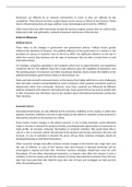
Example:
This DAG says that people who smoke are more likely to carry a lighter and to be
healthy and people with more education are less likely to have a lighter and are
more likely to be healthy. There are 3 paths between lighter and health: 1 causal
path between lighter and health and 2 backdoor paths through smoking and
education. The 3 together explain why lighter and health are associated. When
you want to adjust for education because there is a pure association of lighter
and health or lighter and health are independently associated, then the
association is a meaningless mixture of causal and non-causal elements. Lighter
and health are associated because of smoking.
Collider bias
Conditioning on common effect. When you adjust for a collider, this path will be opened where there is
none causal inference. So never adjust for a collider, never stratify on it and do not select a sample based
on a collider.
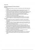
Example:
You want to know the association between a diet and a disease. Both people who
are following a diet and people with a disease are more likely to lose weight. If
the DAG is correct than we have 1 path (non-casual path) between diet and
disease and that goes through weight loss = collider. You cannot adjust for weight
loss because it is a collider. It would lead to false outcomes if you adjust for
weight loss.
Selection bias = collider bias
Quantitative part
Lecture 1
Epidemiology: Methodology and philosophy about causal relationships.
Causal inference
Causation: In an individual, a treatment has a causal effect if the outcome under treatment 1
would be different from the outcome under treatment 2.
Causal effect: A leads to B, the exposure leads to the outcome. ‘Influences or improve’ investigate
a causal effect. For example, the ad of L’Oréal says that using L’Oréal true match
mineral leads to a better skin.
𝑌𝑖𝑎=1 ≠ 𝑌𝑖𝑎=0
Y=outcome, a=treatment, 1= yes, 0= no, i= individual, ≠ does not equal
No causal conclusion can be drawn when: the research group is too small, commercial organization makes
statements, and no control group is present. Individual causal effect cannot be observed → missing data
problem.
We can determine average outcome effects under:
- No assumptions (RCT)
- Very strong assumptions (observational studies)
Outcomes
Not all potential outcomes are observed, there are two types of outcomes:
Counterfactual outcome: Potential outcome that is not observed because the subject did not
experience the treatment (counter the fact). It is important to observe the
counterfactuals because then you what would have happened if a patient did
not use a treatment.
𝑎=1
Potential outcome (𝑌𝑖 ): Factual for some subjects, and counterfactual for others.
Based on the population averages, conclusions on causal effects can be drawn if three identifiability
conditions hold:
- Positivity: You need data for all treatments in the case to see the difference between treatment
and no treatment, you can use a control group to see. Observe; what would have
happened if..
- Consistency: The treatment and no treatment must be described in detail (define ‘if’)
- Exchangeability: The two groups receiving treatment and no treatment must be
exchangeable, so randomize. Potential outcomes are independent of the treatment
that was actually received. Observe; what would happened if.. It is necessary to
consider (adjust); if within the smoking group; are people with and without lighter
exchangeable?
→ Association can be ascribed (=toegeschreven) to treatment effect
RCT
If the conditions are met, then association of exposure and outcome is unbiased estimate of causal effect.
The best way to hold on to the three assumptions needed for drawing conclusions on causal effects, is a
Randomized Controlled Trial (RCT). You select your patients, randomly assign them to treatment groups
and define a golden standard for treatment.
Observational study
When RCT are not possible or when the people in the trial are different from the world outside.
+ Leads to real world outcomes
+ A lot of data is available
- Internal validity threatened by lack of exchangeability
- Positivity and consistency need explicit attention.
,Association does not equal causation
Causal conclusions can be drawn if identifiability conditions are true, to see what assumptions are required
we use:
- Theory/knowledge
- Causal structure
- Adjustment to improve exchangeability
Adjustment
Complete and correct adjustment leads to exchangeability, ways to do:
• Stratification
• Matching
• Weighting
• Regression analysis
Stratification
Association: people with cigarette lighters less likely to be healthy.
Total sample With lighter (n=110) Without lighter (n=190)
Healthy 63 (57%) 165 (87%)
Smokers With lighter (n=90) Without lighter (n=10)
Healthy 45 (50%) 5 (50%)
→ stratum where the groups (with and without lighter) are both 50% healthy.
After adjusting (what is only possible with positivity) we achieve exchangeability and, then a causal
conclusion can be made. Adjustment for exchangeability!
How do you select variables that need to be adjusted?
• Stepwise: start with all variables and remove one by one the variable that is least statistically
significant, leave in variable if removal leads to substantial change in the estimate of the treatment
effect
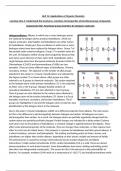
• Adjust for confounders. Confounders are:
- Associated with the exposure (people with a lighter are more likely to smoke, lighter is the
exposure and smoking the association).
- Conditionally associated with the outcome
(health), given the exposure
- Are not in the causal path between exposure
and outcome
Problems with these strategies of selecting variables for
adjusting:
They rely on the observed data rather than on a priori
knowledge of causal structures
- Data must have been collected, strategy cannot
be used in the design
- Important variables may be missed
- They might increase bias rather than reduce it
Solutions → Directed Acyclic Graphs (DAG)
DAG’s graphical represent of underlying causal structures, they encode a priori causal knowledge. A
connection → transmit association. Everything that is connected by arrows, is also associated in the data.
Simple rules can be used to determine what variables to adjust for:
, DAG terminology
- Path: A connection between exposure and outcome, it does not have to follow the
direction of the arrows.
- Backdoor path: A connection between 2 variables, that not follow the direction of the arrows
- Causal path: A connection between 2 variables, that follow the direction of the arrows
- Confounding: Bias caused by common cause of exposure and outcome
- Confounder: A variable that is associated with the exposure, and conditionally associated with the
outcome, given the exposure. Are not in the causal pathway between exposure and
outcome. Variable that can be used to remove confounding (solves the problem of
confounding)
- Collider: A variable where 2 arrows come together
- Blocking: An open path is blocked when we adjust for a variable along the path. You don’t
want bias in your outcome, so you need to block the path with a confounder.
Removing a backdoor path
- Unblocking: Adjusting for a collider. Opening a backdoor path. Collider on a path → closed. Never
adjust a collider, you can correct a collider but then you introduce bias. You just want
to know the path between E and O.
- Open/closed path: All paths are open unless arrows collide somewhere along the path.
All paths are open unless they are adjusted or collide somewhere along the path. Then it doesn’t
contribute to the studied association anymore. Adjusting for a collider, leads to unblocking of the pathway,
that’s not what you want, because then you haven’t isolated the causal inference. Causal inference means
stripping away the association of non-causal elements by blocking backdoor paths. To block backdoor
paths, you need to have data about this variable. In the case of the lighter, you will have to adjust for
smoking to be able to draw a conclusion about lighters and health. If no data on smoking is available, no
causal conclusion can be drawn.
Example:
This DAG says that people who smoke are more likely to carry a lighter and to be
healthy and people with more education are less likely to have a lighter and are
more likely to be healthy. There are 3 paths between lighter and health: 1 causal
path between lighter and health and 2 backdoor paths through smoking and
education. The 3 together explain why lighter and health are associated. When
you want to adjust for education because there is a pure association of lighter
and health or lighter and health are independently associated, then the
association is a meaningless mixture of causal and non-causal elements. Lighter
and health are associated because of smoking.
Collider bias
Conditioning on common effect. When you adjust for a collider, this path will be opened where there is
none causal inference. So never adjust for a collider, never stratify on it and do not select a sample based
on a collider.
Example:
You want to know the association between a diet and a disease. Both people who
are following a diet and people with a disease are more likely to lose weight. If
the DAG is correct than we have 1 path (non-casual path) between diet and
disease and that goes through weight loss = collider. You cannot adjust for weight
loss because it is a collider. It would lead to false outcomes if you adjust for
weight loss.
Selection bias = collider bias