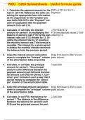
WGU - C268 Spreadsheets - Useful formula guide

WGU - C268 Spreadsheets - Useful formula guide 1. 1. Calculate the payment amount for the loan in cell C15. Reference the cells con- taining the appropriate loan information as the arguments for the function you use. Cells C20-C67 in the "Payment" col- umn are populated with the payment amount from cell C15. 2. Calculate, in cell D20, the interest amount for period 1 by multiplying the balance in period 0 (cell F19) by the loan interest rate (cell C13) divided by 12. Di- viding the interest rate by 12 results in the monthly interest rate. This formula is reusable. The interest for a given period is always the monthly interest rate times the balance from the previous period. 3. Copy the interest amount calculation down to complete the "Interest" column of the amortization table. [2 points] 4. Calculate, in cell E20, the principal amount for period 1. The principal amount is the difference between the payment amount (cell C20) and the inter- est amount (cell D20) for period 1. Con- struct your formula in such a way that it can be reused to complete the "princi- pal" column of the amortization table. 5. Copy the principal amount calculation down to complete the "principal" column of the amortization table. 6. Calculate, in cell F20, the balance for period 1. The balance is the difference between the balance for period 0 (cell F19) and the principal amount for peri- PMT=(c13/12,c12,c11) Payment =F19*$C$13/12 F19 time absolute values C13 di- vided by 12. Drag D19 down to D67 to com- plete column =C20-D20 Drag E20 down to E67 to com- plete column =C20-D20 2 / 10 WGU - C268 Spreadsheets - Useful formula guide od 1 (cell E20). This formula is reusable. The balance is always calculated as the difference between the balance from the previous period and the principal amount for the current period. 7. Copy the balance amount calculation down to complete the "Balance" column of the amortization table. 8. Calculate, in cell G12, the total amount paid by multiplying the payment amount (cell C15) by the term of the loan (cell C12). 9. Calculate the total interest paid in cell G13. The total interest paid is the sum of all interest paid in the "Interest" column of the amortization table. 10. To verify that the total interest calcula- tion from the amortization table is cor- rect, calculate the total interest paid in cell G14. This is the difference between the Total Amount Paid over the course of the loan and the original Loan Amount. Notice the negative sign associated with the original Loan Amount. 11. Assume you have made the first 36 pay- ments on your loan. You want to trade the car in for a new car. You believe that you can sell your car for $4000. Will this cover the balance remaining on the car in period 36? Answer either "Yes" or "No" in cell G15 from the drop-down menu. 12. Use the HLOOKUP function to complete the "Hourly Wage" column of table 1. Use the "Employee" from table 1 as the drag F20 down to F67 to com- plete column =C15*C12 =SUM(D20:D67) Add D20 range through D67 =G12--C11 two minus cancel out the minus from C11 No G36 = 5,193.87 $4,000 is not enough =hlookup(D16, $E$11:$H$12, 2, 0) 3 / 10 lookup_value and the "Employee Wage Information" above table 1 as your refer- ence table. 13. Use the AND function to complete the "Time Bonus?" column of table 1. An em- ployee earns a time bonus if the project's "Hours Worked" are fewer than the "Es- timated Hours" and if the work "Quality" is greater than 1. 14. Use the OR function to complete the "Outcome Bonus?" column of table 1. An employee earns an outcome bonus if the difficulty of a job is greater than 3 or if the quality of their work is equal to 3. 15. Use the IF function to complete the "Time Bonus $" column of table 1. If an employee earns a time bonus (i.e., the corresponding cell in the "Time Bonus?" column is TRUE), then "Time Bonus $" is the "Job Pay" for that project times the bonus percentage in cell M11. Otherwise "Time Bonus $" is 0. 16. Use the IF function to complete the "Out- come Bonus $" column of table 1. If an employee earns an outcome bonus (i.e., the corresponding cell in the "Out- come Bonus?" column is TRUE), then "Outcome Bonus $" is the "Job Pay" for that project times the outcome bonus percentage in cell M12; otherwise, "Out- come Bonus $" is 0. 17. Use the IF function to complete the "Comments" column of table 1. Display "Good Job" if both the "Hours Worked" horizontal lookup (Jim, absolute value E and 11 through absolute value H and 12, 2nd column, Ex- act) =AND(E16C16,H161) And used when all logical func- tions are true. (E16 greater than C16, AND H16 greater than 1) =OR(G163,H16=3) when either logical functions need to be true. (G16 greater than 3, OR H16=3 =IF(I16=TRUE,K16*$M$11,0) IF I16 is true, it will *.010, if not, it will display false. =IF(J16=True, K16*$M$12,0) IF J16 is true, it will *.010 the Out come percentage bonus =- IF(AND(E16=C16,H161),"Good Job",IF(E16C16,"Too Much 4 / 10 are less than or equal to the "Estimated Hours" for a project and the assessed "Quality" of that project is greater than 1. Display "Too Much Time" if the "Hours Worked" on a project exceed the "Esti- Time","Poor Quality")) IF E16 is less than or equal to C16 AND H16 is greater than one, "Good Job", IF E16 mated Hours" for that project; otherwise, is greater than C16, "Too much display "Poor Quality" in the cell. 18. Use the VLOOKUP function to complete time, other wise display "Poor Quality" =- the "Employee" column of table 2. Use VLOOKUP(B40,$B$16:$D$35,3,FAL "Job ID" from table 2 as your lookup_val- ue(s) and table 1 as the reference table. 19. Use the VLOOKUP function to com- plete the "Difficulty" column of table 2. Again, use "Job ID" from table 2 as the lookup_value(s) and table 1 as the refer- ence table. 20. Use the COUNTIF function to complete the "# of Jobs" column in table 3. Ref- erence the appropriate field in table 1 as your range and the "Employee" names in table 3 as your criteria. 21. Use the SUMIF function to complete the "Total Hours" column in table 3. Refer- ence the appropriate field in table 1 as your range and the "Employee" names in table 3 as your criteria. 22.22. Vertical lookup, Find value of B40 in table B16 through D35, look at the 3rd column, find exact match =- VLOOKUP(B40,$B$16:$G$35,6,FA Vertical lookup, Find value in B40, search for it in B16 through G35, look at 6th column, find ex- act match =COUNTIF($D$16:$D$35,G39) Counts the occurrences in range D16-D35, looks for the value in G39. =- SUMIF($D$16:$D$35,G39,$E$16:$ Adds the absolute range of D16-D35, looks for the value in G39, and adds the hours of ab- solute range of E16-E35 5 / 10 Use the SUMIF function to complete the =- "Total Pay" column in table 3. Reference SUMIF($D$16:$D$35,G39,N16:N35 the "Employee" field in table 1 as your range, the "Employee" names in table 3 as your criteria, and the "Total Pay" field in table 1 as your sum_range. 23. Use the COUNTIF function to complete the "# of Touch-ups" column in table 4. Reference the appropriate field in table 2 as your range and the "Difficulty" rating in table 4 as your criteria. 24. Use the SUMIF function to complete the "Cost Touch-ups" column in table 4. Ref- erence the appropriate field in table 2 as your range and the "Difficulty" rating in table 4 as your criteria. 25. Use the AVERAGEIF function to com- plete the "Average Hours/Job" column in table 4. Reference the appropriate field in table 1 as your range and the "Difficulty" rating in table 4 as your criteria. 26. Construct a column chart to examine the total annual revenue for Google, Inc. from 2003 to 2010, using the data in looks in table range D16-D35, looks for value from G39, Adds the number from table range N16-N35 =COUNTIF($D$40:$D$46,G46) Formula looks at absolute rang of D40-D46, for value in G46 =(- SUMIF($D$40:$D$46,G46,$E$40:$ Formula looks at table range D40-D46, looks for value in G46, and then looks at E40-E46 =AVER- AGEIF($G$16:$G$35,G46,$E$16:$ Gets the average of values in G16-G35, for value in G46, aver- ages values in E16-E35 Highlight C12-J12 Select "Insert" from the top Rib- bon menu table 1 (range C12:J12). Format the chart Insert a 2D Column Chart with the title "Total Google Revenue" and the years across the horizontal axis. Do not include a legend. Note: in order for the grading engine to identify the chart for grading, the title must be precise- ly, "Total Google Revenue" (without the quotes). Rename the chart name to Total Google Revenue Single click chart, click the Filter icon on the right, click select data on pop-up menu, click EDIT in the horizontal axis labels Select the range C7-J7 to fill in 6 / 10 27. Construct a stacked column chart to the data in the Axis Range win- dow. Highlight B8-J11 compare the revenue totals for each year, Select "Insert" from the top Rib- using the quarterly revenue totals (range C8:J11). Format the chart with the title "Google Revenue by Quarter", the year as the horizontal axis, and a legend that depicts each quarter using the text la- bels provided in the tables. Do not in- clude the total annual revenue (range C12:J12) in the chart. Note: in order for the grading engine to identify the chart for grading, the title must be precisely, "Google Revenue by Quarter" (without the quotes). 28. Use the LEN function in cell D10 to de- termine the number of characters in the statement template in cell D9 29. Use the SEARCH function in cell D11 to determine the position of the "#" charac- ter in the statement template (cell D9). 30. Use the SEARCH function in cell D12 to determine the position of the "$" charac- ter in the statement template (cell D9). bon menu Insert a 2D column Stacked chart Rename chart to Google Rev- enue by Quarter Single click chart, click the Filter icon on the right, click select data on pop-up menu, click EDIT in the horizontal axis labels Select the range C7-J7 to fill in the data in the Axis Range win- dow. Ensure you have the legend dis- played at the bottom of chart. =LEN(D9) 28 =SEARCH("#",D9) 23 Searches for the # sign in cell D9 and displays position of charac- ter =SEARCH("$",D9) 9 Searches for the $ sign in cell D9 and displays position of charac- ter 7 / 10 31. Use the LEFT function in cell D13 to re- turn the text "I spent $" from the state- ment template in cell D9. Refer to the location of the "$" character you calcu- lated in cell D12 as the "num_char" argu- ment for your function. 32. Use the MID function in cell D14 to return the text "at merchant #" from the state- ment template in cell D9. Refer to the location of the "$" (in cell D12)—adjust- ed by adding 1—as the "start_num" ar- gument. Use the difference between the location of the "#" character (in cell D11) =LEFT(D9,9) I spent $ Looks at D9 starting from the LEFT to display the first 9 char- acters =MID(D9,10,14) at merchant # Searches the middle of D9, dis- plays the characters in at posi- tion 10 and number of characters and the "$" character (in cell D12) as the you want to display "num_char" argument. 33. Use the RIGHT function in cell D15 to return the text "on:" from the statement template in cell D9. Use the difference between the length of the statement tem- plate (in cell D10) and the location of the "#" character (in cell D11) as the "num_char" argument. 34. Use the MONTH function in cell E18 to calculate the month portion of the "Time Stamp" in cell B18. Copy and paste your function down to complete the "Month" column of the table. 35. Use the DAY function in cell F18 to calcu- late the day portion of the "Time Stamp" in cell B18. Copy and paste your function down to complete the "Day" column of the table. =Right(D9,5) on: Examines D9 from the right, to display up to 4 characters =month(B18) Excel apparently knows what to do with the data in B18 Drag down to the bottom of table to reveal all "8s" (for August). =day(B18) Excel apparently knows what to do with the data in B18. Drag the formula down to the bot- tom of the column DAY. 8 / 10 36. Use the HOUR function in cell G18 to calculate the hour portion of the "Time Stamp" in cell B18. Copy and paste your function down to complete the "Hour" column of the table. 37. Use the MINUTE function in cell H18 to calculate the minute portion of the "Time Stamp" in cell B18. Copy and paste your function down to complete the "Minute" column of the table. 38. Use the SECOND function in cell I18 to calculate the second portion of the "Time Stamp" in cell B18. Copy and paste your function down to complete the "Second" column of the table. 39. Use the CONCAT function (or the CON- CATENATE function if you are using Ex- cel 2013 or earlier) in cell J18 to create the "Date" by combining the "Month" in cell E18 with the "Day" in cell F18. "Date" should use this syntax: "Month/Day." Your function should, therefore, also insert the "/" character between the "Month" and "Day." Copy and paste your formula down to complete the "Date" col- umn of the table. 40. Use the CONCAT function (or the CON- CATENATE function if you are using Ex- cel 2013 or earlier) to create the "Trans- action Statement" in cell K18. The state- ment in cell K18 should read "I spent =Hour(b18) Excel apparently knows what to do with the data in B18. Drag the formula down to the bot- tom of the column HOUR. =minute(b18) Excel apparently knows what to do with the data in B18. Drag the formula down to the bot- tom of the column MINUTE. =SECOND(B18) Excel apparently knows what to do with the data in B18. Drag the formula down to the bot- tom of the column SECOND. =concatenate(E18,"/",F18) Combines date in E18, separat- ed by a /, and data in F18 =CONCATE- NATE($D$13,D18,$D$14,C18,$D$1 9 / 10 $24.06 at merchant #4931 on: 8/1". To make this statement, combine "State- ment P1" in cell D13, the "Amount" in cell D18, "Statement P2" in cell D14, the "Merchant ID" in cell C18, "Statement P3" in cell D15, and the "Date" in cell J18. Copy and paste your function down to complete the "Transaction Statement" column of the table. [ 41. In the "Input Analysis" section of the spreadsheet model, calculate the aver- age attendance and sales for each type of product from the past events listed in the "Past Events" worksheet. 42. In the "Input Analysis" section of the Combines, absolute D13, with D18, and absolute D14, and C18, and absolute D15, and J18. =AVERAGE('Past Events'!C4:C103) =AVERAGE('Past Events'!D4:D103) =AVERAGE('Past Events'!E4:E103) =AVERAGE('Past Events'!F4:F103) =STDEV.S('Past spreadsheet model, calculate the sample Events'!C4:C103) standard deviation for attendance and sales for each type of product from the past events listed on the "Past Events" worksheet. (Note for Excel 2007 users: Excel 2007 does not support a specif- ic function to calculate sample standard deviations. Use the STDEV function in- stead.) 43. In the "Input Analysis" section of the spreadsheet model, calculate the 95% confidence interval for the sales for each type of product. (You will not calculate a confidence interval for attendance.) Use the number of events (calculated in cell I3) as part of your calculations. 44. In the "Input Analysis" section of the spreadsheet model, calculate the corre- =STDEV.S('Past Events'!D4:D103) =STDEV.S('Past Events'!E4:E103) =STDEV.S('Past Events'!F4:F103) =CONFI- DENCE.NORM(0.05,J7,$I$3) =CONFI- DENCE.NORM(0.05,K7,$I$3) =CONFI- DENCE.NORM(0.05,L7,$I$3) =CORREL('Past Events'!$C$4:$C$103,'Past 10 / 10 lations between the sales of each type of product and event attendance. Use ap- propriate ranges from the "Past Event" worksheet for your calculations. 45. The sales for which product type are most highly correlated with attendance? Select the correct answer from the drop-down list in cell L32. 46. In the "Input Analysis" section of the spreadsheet model, calculate a sales forecast for each type of product if ex- pected attendance at the future event is 18000 people. Reference cell I13 (the at- tendance forecast) for your calculations. Events'!D4:D103) =CORREL('Past Events'!$C$4:$C$103,'Past Events'!E4:E103) =CORREL('Past Events'!$C$4:$C$103,'Past Events'!F4:F103) Food Close to 1.00 =FORECAST($I$13,'Past Events'!D4:D103,'Past Events'!C4:C103) =FORECAST($I$13,'Past Events'!E4:E103,'Past Events'!C4:C103) =FORECAST($I$13,'Past Events'!F4:F103,'Past Events'!C4:C103) Remember your X value for the forecast formula should match the X data type, example At- tendance and past Attendance numbers. =forcase(X,knownY, knownX)