
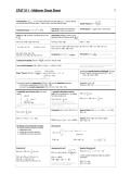
STAT 511 - Midterm Cheat Sheet 1
Trimmed Mean: (%)Given · n = # of values deducted from both sides (nR) → remove highest Σ(𝑥𝑖−𝑥)
2
and lowest values from both ends → reduce n by nR and then take the mean Sample Variance: s2 =
𝑛−1
2 Lower Fourth: median of the smallest half Fourth Spread: fs = upper fourth - lower fourth
Standard Deviation: s = σ = 𝑠 = 𝑉(𝑋) Upper Fourth: median of the largest half
Union (A ∪ B): consists of all elements in A and Intersection (A ∩ B): consists of only
B; “or” elements that are in both A and B; “and”
P(A ∪ B) = P(A) + P(B) - P(A ∩ B) P(A ∩ B) = P(A) · P(B) P(A’) = 1 - P(A)
(A ∪ B)’ = A’ ∩ B’ (A ∩ B)’ = A’ ∪ B’ P(A ∪ B ∪ C) = P(A) + P(B) + P(C) - P(A ∩ B) - P(A ∩ C) - P(B ∩ C) + P(A ∩ B ∩ C)
P (A ∩ B ∩ C) = P(A) · P(B) · P(C)
P(A ∩ B’) = P(A) - P(A ∩ B) 𝑛 𝑛!
Permutation: nPr = (𝑛−𝑟)!
𝑛!
Combination: nCk = ( ) = 𝑘!(𝑛−𝑘)! *the way a set can be ordered
P(A ∩ B ∩ C’) = P(A ∩ B) - P(A ∩ B ∩ C) 𝑘
𝑃(𝐴 ∩ 𝐵)
Conditional Probability: P(A⏐B) = 𝑃(𝐵)
, P(A ∩ B) = P(A⏐B) · P(B)
Law of Total Probability: P(B) = P(B⏐A1) · P(A1) + … + P(B⏐Ak) · P(Ak) *used to find the probability of an event when you don’t know enough
about the event’s probability to calculate it directly
𝑃(𝐴𝑗 ∩ 𝐵) 𝑃(𝐵⏐𝐴𝑗)·𝑃(𝐴𝑗) A and B are mutually exclusive (disjointed) if A and
Bayes’ Theorem: P(Aj⏐B) = = 𝑘 , j = 1, …, k B cannot happen simultaneously and P(A ∩ B) = 0
𝑃(𝐵)
∑ 𝑃(𝐵⏐𝐴 ) · 𝑃(𝐴𝑖) - P(A ∪ B) = P(A) + P(B)
𝑖
𝑖=1
*used to find posterior probabilities using prior probability distributions *used when asked either A or B
Two events A and B are independent if P(A⏐B) = P(A) and are dependent otherwise. P(parallel) = P(A ∪ B)
- If A and B are independent, P(A ∩ B) = P(A) · P(B): P(series) = P(A ∩ B) *think of it like a circuit in physics
- A, B, and C are mutually independent if P(A ∩ B ∩ C) = P(A) · P(B) · P(C)
A probability mass function (pmf), p(x), must A cumulative distribution function 𝑎
satisfy: (cdf), F(x), of a discrete rv X is defined P(X ≤ a) = ∑ 𝑝(𝑦)
𝑦=1
1. p(x) ≥ 0 for every number x by: 𝑎
P(X ≥ a) = 1 - P(X < a) = 1 - ∑ 𝑝(𝑦)
2. ∑ 𝑝(𝑥) = 1 F(x) = P(X ≤ x) = ∑ 𝑝(𝑦) 𝑦=1
𝑎𝑙𝑙 𝑝𝑜𝑠𝑠𝑖𝑏𝑙𝑒 𝑥 𝑦≤𝑥
3. P(X = x) = p(x) *used to determine the probability that a random
*specifies probability of observing value when experiment is observation taken from the population will be less than
performed or equal to a certain value
𝑏 Proposition: P(a ≤ X ≤ b) = F(b) - F(a - 1) Expected Value: E(X) = 𝜇x = x1, · P(x1) + … + xn · P(xn)
P(a ≤ X ≤ b) = ∑ 𝑝(𝑦) E(X) = np
𝑦=𝑎
E(X2) = x12 · P(x1) + … + xn2 · P(xn) Variance: V(X) = E[(X - 𝜇)2] = E(X2) - (E(X))2
E[h(X)] = 𝜇h(X) = ∑ ℎ(𝑥) · 𝑝(𝑥) = h[E(X)] V(X) = np(1 - p)
Identifying a Binomial Random Variable: Binomial pmf:
B - binary outcome (success or failure)
I - independent trials
n - sample size is fixed in advance
S - probability of success is given, p
E(X) = np V(X) = np(1 - p) σx = 𝑛𝑝(1 − 𝑝)
Binomial cdf: Hypergeometric pmf: Negative Binomial pmf:
𝑥 𝑀 𝑁−𝑀 𝑥+𝑟−1 𝑟 𝑟
( 𝑥 )( 𝑛 − 𝑥 ) nb(x; r, p) = ( ) · 𝑝 · (1 − 𝑝)
B(x; n, p) = P(X ≤ x) = ∑ 𝑏(𝑦; 𝑛, 𝑝) 𝑟 −1
𝑦=0 P(X = x) = h(x; n, M, N) = 𝑁
(𝑛 )
x is the number of failures it takes to achieve r
P(X = a) = P(X ≤ a) - P(X ≤ (a - 1)) E(X) = n · (M/N) successes
P(X ≥ a) = 1 - P(X ≤ (a - 1)) V(X) =
𝑁−𝑛
·𝑛
𝑀
· (1 −
𝑀
)
𝑁−1 𝑁 𝑁
P(a ≤ X ≤ b) = P(X ≤ b) - P(X ≤ (a - 1)) E(X) = r(1 - p)/p
*used to determine probability of obtaining a certain V(X) = r(1 - p)/p2
number of successes without replacement
Trimmed Mean: (%)Given · n = # of values deducted from both sides (nR) → remove highest Σ(𝑥𝑖−𝑥)
2
and lowest values from both ends → reduce n by nR and then take the mean Sample Variance: s2 =
𝑛−1
2 Lower Fourth: median of the smallest half Fourth Spread: fs = upper fourth - lower fourth
Standard Deviation: s = σ = 𝑠 = 𝑉(𝑋) Upper Fourth: median of the largest half
Union (A ∪ B): consists of all elements in A and Intersection (A ∩ B): consists of only
B; “or” elements that are in both A and B; “and”
P(A ∪ B) = P(A) + P(B) - P(A ∩ B) P(A ∩ B) = P(A) · P(B) P(A’) = 1 - P(A)
(A ∪ B)’ = A’ ∩ B’ (A ∩ B)’ = A’ ∪ B’ P(A ∪ B ∪ C) = P(A) + P(B) + P(C) - P(A ∩ B) - P(A ∩ C) - P(B ∩ C) + P(A ∩ B ∩ C)
P (A ∩ B ∩ C) = P(A) · P(B) · P(C)
P(A ∩ B’) = P(A) - P(A ∩ B) 𝑛 𝑛!
Permutation: nPr = (𝑛−𝑟)!
𝑛!
Combination: nCk = ( ) = 𝑘!(𝑛−𝑘)! *the way a set can be ordered
P(A ∩ B ∩ C’) = P(A ∩ B) - P(A ∩ B ∩ C) 𝑘
𝑃(𝐴 ∩ 𝐵)
Conditional Probability: P(A⏐B) = 𝑃(𝐵)
, P(A ∩ B) = P(A⏐B) · P(B)
Law of Total Probability: P(B) = P(B⏐A1) · P(A1) + … + P(B⏐Ak) · P(Ak) *used to find the probability of an event when you don’t know enough
about the event’s probability to calculate it directly
𝑃(𝐴𝑗 ∩ 𝐵) 𝑃(𝐵⏐𝐴𝑗)·𝑃(𝐴𝑗) A and B are mutually exclusive (disjointed) if A and
Bayes’ Theorem: P(Aj⏐B) = = 𝑘 , j = 1, …, k B cannot happen simultaneously and P(A ∩ B) = 0
𝑃(𝐵)
∑ 𝑃(𝐵⏐𝐴 ) · 𝑃(𝐴𝑖) - P(A ∪ B) = P(A) + P(B)
𝑖
𝑖=1
*used to find posterior probabilities using prior probability distributions *used when asked either A or B
Two events A and B are independent if P(A⏐B) = P(A) and are dependent otherwise. P(parallel) = P(A ∪ B)
- If A and B are independent, P(A ∩ B) = P(A) · P(B): P(series) = P(A ∩ B) *think of it like a circuit in physics
- A, B, and C are mutually independent if P(A ∩ B ∩ C) = P(A) · P(B) · P(C)
A probability mass function (pmf), p(x), must A cumulative distribution function 𝑎
satisfy: (cdf), F(x), of a discrete rv X is defined P(X ≤ a) = ∑ 𝑝(𝑦)
𝑦=1
1. p(x) ≥ 0 for every number x by: 𝑎
P(X ≥ a) = 1 - P(X < a) = 1 - ∑ 𝑝(𝑦)
2. ∑ 𝑝(𝑥) = 1 F(x) = P(X ≤ x) = ∑ 𝑝(𝑦) 𝑦=1
𝑎𝑙𝑙 𝑝𝑜𝑠𝑠𝑖𝑏𝑙𝑒 𝑥 𝑦≤𝑥
3. P(X = x) = p(x) *used to determine the probability that a random
*specifies probability of observing value when experiment is observation taken from the population will be less than
performed or equal to a certain value
𝑏 Proposition: P(a ≤ X ≤ b) = F(b) - F(a - 1) Expected Value: E(X) = 𝜇x = x1, · P(x1) + … + xn · P(xn)
P(a ≤ X ≤ b) = ∑ 𝑝(𝑦) E(X) = np
𝑦=𝑎
E(X2) = x12 · P(x1) + … + xn2 · P(xn) Variance: V(X) = E[(X - 𝜇)2] = E(X2) - (E(X))2
E[h(X)] = 𝜇h(X) = ∑ ℎ(𝑥) · 𝑝(𝑥) = h[E(X)] V(X) = np(1 - p)
Identifying a Binomial Random Variable: Binomial pmf:
B - binary outcome (success or failure)
I - independent trials
n - sample size is fixed in advance
S - probability of success is given, p
E(X) = np V(X) = np(1 - p) σx = 𝑛𝑝(1 − 𝑝)
Binomial cdf: Hypergeometric pmf: Negative Binomial pmf:
𝑥 𝑀 𝑁−𝑀 𝑥+𝑟−1 𝑟 𝑟
( 𝑥 )( 𝑛 − 𝑥 ) nb(x; r, p) = ( ) · 𝑝 · (1 − 𝑝)
B(x; n, p) = P(X ≤ x) = ∑ 𝑏(𝑦; 𝑛, 𝑝) 𝑟 −1
𝑦=0 P(X = x) = h(x; n, M, N) = 𝑁
(𝑛 )
x is the number of failures it takes to achieve r
P(X = a) = P(X ≤ a) - P(X ≤ (a - 1)) E(X) = n · (M/N) successes
P(X ≥ a) = 1 - P(X ≤ (a - 1)) V(X) =
𝑁−𝑛
·𝑛
𝑀
· (1 −
𝑀
)
𝑁−1 𝑁 𝑁
P(a ≤ X ≤ b) = P(X ≤ b) - P(X ≤ (a - 1)) E(X) = r(1 - p)/p
*used to determine probability of obtaining a certain V(X) = r(1 - p)/p2
number of successes without replacement