

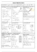
ELECTROSTATICS
1 Q N dV 1 Q J
Electric Field Intensity:- E = vector unit:- E=− Electric Potential V = scalar unit:- V = − E.dr
40 r 2 C dr 40 r C
Electric Dipole:- Equal and Opposite charge separated by small distance, Dipole moment P = 2ql vector(direction from negative to positive charge unit:- C m
E & V on Equitorial line:- Torque on Dipole:- Net force = +qE – qE = 0
E & V on Axial Line:- E at pt. P on axial line Torque = Force × ⊥ distance
E = EA cos + EB cos
= qE × BC [BC = 2l × sin θ
since = qE 2l sin θ
= E (2ql) sin θ
is E = E B + ( −E A ) EA = EB
τ = PE sin θ = P E
1 q 1 q E = 2EA cos τmax = PE for θ = 90o
E= −
40 ( r − l )2 40 ( r + l )2 work done in Rotating Dipole
1 q l l
E=
q 1
−
1
40 ( r − l )2 ( r + l )2
E = 2
2ql
40 x2 x
P
cos =
x W=
d = (1 − cos ) PE
E= = Energy of Dipole: U = –PE cos θ
40x3 ( )
3 Stable equilibrium θ = 0, U= –PE
2 2qrl 2pr 40 x2 + l2
E= = Unstable equilibrium
40 ( r2 − l2 ) 40 ( r2 − l )
2 2
P Θ = 180o ⇒ U = PE.
E=
3
40 ( r2 + l2 ) 2
2P Gauss Theorem:- Total electric flux (total no. of lines
E= For short dipole r >> l (direction (-)
3
40r of forces) emerges from closed surface is
1
times the
P 0
to (+)) E= For short dipole r >> l
40 ( r3 )
E.dS =
qin
1 −q 1 q Direction (+) to (-) charge enclosed
V = VA + VB = +
40 ( r + l ) 40 ( r − l ) 1 ( −q )
0
1 q
V = VA + VB = + =0
P 40 x 40 x
1 P
= V=
40 ( r2 − l2 ) 4 r2 0
E due to long charged wire: E due to charged plane sheet: E due to charged Hallow Sphere:
q q q
Linear charge density = Surface charge density = Volume charge density =
l A V
E.dS =
qin For non conducting plate charge is on both side
E.dS =
qin
q
0 2 E.dS = 0
0
E.dS + E.dS + E.dS =
qin
q
1 2 3 E dS =
q 0
0 2EA =
For dS2 and dS3 θ = 90 o 0
E( 4r2 ) =
q
For curved surface dS1 θ = 0 q
E= E= 0
q q
E dS = ⇒ E ( 2rl ) = 20 A 20
0 0 E=
1 q
On surface
40 R 2
2q For conducting sheet E =
0
q 1 2 1 q
E= = l ⇒E= * E is independent of distance from the sheet. E= Outside & E = 0 as q = 0 inside
2rl0 40r 40 r 40 r2
Capacitor:- Q = CV unit:- Farad, * C depends on dimensions
Capacitance for parallel plate Surface charge Density Energy of Capacitor
capacitor Q
= Q = A
Energy = work done in bringing charge
Consider || plate capacitor with A at potential V
area of plate A, capacitance C and Electric field q
dW = V dq = .dq
dist. b/w plates d E = Eair + Edielectric C
Q Q Q
C=
Q
=
Q 1 q2 1 Q2
= +
1
V Ed 0 k0 U = dW = q dq = =
C C 2 0 2 C
0 0
E= for charged sheet Potential V = E × d
0 1Q 1 2
1
( U= = CV 2 = QV
V = a + b) + t 2 C 2 2
=
Q
for surface charge density 0 k0
A Energy Density (energy per unit volume)
t
A A V= a + b + 1 2 1 0 A (
E d)
2
C= = 0 0 k CV
1
d
d = 2 =2 d = 0E2
0 t volume Ad 2
V= d − t +
0 k Unit of energy density:- J/m3
If dielectric with dielectric
Q A
constant k is filled b/w the plates. Now C= =
V t
C’ = kC d − t +
0 k
, CURRENT ELECTRICITY
q A – Area
Electric Current: i = , unit - Ampere n – number of free electrons in unit volume
t
nAle RA m
* Scalar quantity i =q/t = resistivity ρ = ρ =
Drift velocity:- v = u + a t l ne2
if u = 0 − relaxation time (10
–14
s) Also J = E
Vd = a Current I = neAVd J=
I
= current density (vector)
eE eV I ne 2 A A
Also ma = eE = f a = I = neA =
m ml V ml
V = IR
eE
Vd = (10–5 m/s) as V = Exl V ml
m R= =
I ne2 A
eV
Vd = V
ml Mobility = d (m2/sV)
E
Temperature dependence of resistivity Electric Energy & power Colour Coding of Resistor
with increase in temperature Power = Energy / Time = Work done / Time
conductors : decrease. inc. It is a scalar quantity
V2
semiconductors; n increase dec E = V.I.t = I 2 Rt = t
R
V2
P = V.I = I 2 R =
R
1 unit = 1 KWh
Series combination of resistance:- R = R1 + R2. Current same E = V + ir charging KIRCHOFF’S LAW
Parallel combination of resistance:- 1/R = 1/R1 + 1/R2 Voltage same E = V – ir discharging i. i = 0 Junction law
ii. iR = E = 0 Voltage law
Cell in series I = nE /nr + R Meter Bridge:
nE Let Unknown Resistance = X
Cell in parallel i=
r + nR R l
=
Wheatstone Bridge: X 100 − l
Balance condition P/Q=R/S R(100 − R)
X=
Potential at A & B same at null pt. l
RA
Position of Galvanometer & Resistivity =
L
battery can be interchanged at null pt.
Meter bridge in most sensitive when null pt. in middle.
Potentiometer:
Principle:- If constant current flows through wire of uniform cross section, then drop in directly proportional to length of that portion
E Advantage of Potentiometer over voltmeter:-
K = = Potential gradient 1. Preferred over voltmeter as it give exact reading draw no
L current
When K1 inserted then E1 = K × L1 2. Sensitivity increase with increase in length
When K2 inserted then E2 = K × L2 3. A small P. D can be measured accurately with the help of
E1 L1 potentiometer. The resistance of voltmeter is high but not
=
E 2 L2 infinity to work as an ideal voltmeter.
4. The internal resistance of a cell can be measured with the
help of potentiometer.
When only K1 is inserted then E = K × L1
When K1 and K2 both are inserted then
V = K × L2 = E – r
l
r = R 1 − 1
l2
, MOVING CHARGES & MAGNETISM
Magnetic Field:- Produced by magnet, moving charge, Vector quantity. Unit:- Tesla (weber/m2), gauss (maxwell/cm2) IT = 104 G
Oested Experiment:- Current carrying conductor produces magnetic field.
Bio Savart Law:- It gives M.F. at a point around
Ampere’s Circuital Law:- B.dl = 0i The line integral of magnetic field B for
current carrying conductor.
idl sin any closed circuit is equal to μ0 times current i threading through this closed loop
dB = 0
4 r 2 and this closed loop is called Amperian loop.
0 B. Due to Infinitely Long Wire:-
= 10−7 TmA−1 Magnetic field at P due to wire
4
μ0 – Permeability of free space
Direction of B:- Perpendicular to dl and r.
B.dl = 0i
B = 0 if sin θ = 0 B dl = 0i
B = max sin θ = 1 θ = 90o
idl r B(2πr) = μ0i
Vector Form dB = 0
4 r 3 2l
B= 0
4 r
Mag. Field At Centre of Coil:-
Direction:- Right Hand Thumb Rule curly finger gives field direction if thumb of
idl sin 90o right hand points current outside
dB = 0
4 r2 B. due to Solenoid:-
B = i
dB = 0 2
4 r
dl
Bdl = B.dl cos
i N – Total Turns
= 0 2 (2r ) d
4 r
i
B = 0 or B = 0
Ni
a
B.dl = 0i
2r 2r
b c d a
Direction:- Right Hand Thumb Rule.
On Axis of Coil:-
0 idl sin 90o
a
b
c
B.dl + B.dl + B.dl + B.dl = 0 ( Ni )
d
dB =
4 x2 b
B = dB sin B.dl + 0 + 0 + 0 = ( Ni )
a
0
0i ( 2a ) a
= . b
4x2
x N
B. dl = 0 Ni B.L = 0 ni ⇒ ∴ B = μ0ni n= (Turns per unit Length)
2 L
0 Nia
B= a
2 ( a2 + r 2 )
3/ 2
Force on charge in Electric field:- Magnetic Field:-
B. Due to Toroid:- (Closed solenoid) F = qE (both for rest & motion) F = qV Bsin θ (only for moving charge)
B.dl = Ni0
B (2r ) = 0 Ni
0 Ni N
B= n =
2 r 2r
B = 0 ni [at P]
Lorentz Force:- F = qE + qvB sin θ = q (E + vB sin θ)
Cyclotron:- Used to accelerate charge Particles. Force b/w 2 parallel current carrying wire:- Force acting on a due to b.
Principle:- The repeated motion of charged particles under mag. & ele. 2i
field accelerates it. E.F. provides energy while M.F. changes direction. F = 0 1 i2l sin 90o
4 r
Construction:- Dees, Sources, M.F., R.F. Oscillator
1 2 2i i
Working:- Max KE = mvmax F = 0 1 2 (For unit Length)
2 4 r
2 By Flemings LHR force is of attraction for same
1 qBr
= m direction of current and force of repulsion for opposite
2 m direction of current.
2 2 2
1q B r if i1 = i2 = 1 A, r = 1m.
K .E. =
2 m then F = 2 × 10⁻⁷ N.
Current Sensitivity:- Deflection per unit current
Moving Coil Galvanometer:- Device Torque Experienced By a BAN Radian
Is = =
to detect & measure electric current. Current loop in uniform i C Ampere
Principle:- Current loop experience Magnetic Field:- Voltage Sensitivity:- Deflection per unit voltage
torque in uniform M.F. τ = F × ⊥ distance
I BAN Radian
Construction:- Light Coil, concave = Bil × bsin θ Vs = s = = =
magnetic Poles → radial field. τ = Bi A sin θ R V iR CR Volt
Theory:- Deflecting torque For N Turns:-
Limitation:- Only charged particles can be acceleration Application:-
= Restring force (torque) τ = BiNa sin θ
For circular path:- For nuclear
B × i × N × A × sin θ = CØ
mv2 mv reaction & other
(θ = 90o) as field is radial = qvB ⇒ r = ⇒r∝v research purpose.
C r qB
∴ B AiN = CØ ⇒ i =
ABN 1 q 2 B2r 2
K .E. =
2 m
Time period = Distance / Velocity = 2πr / v ⇒ T = 2πm / qB
Frequency of Revolution:- f = 1/T = qB/2πm
1 Q N dV 1 Q J
Electric Field Intensity:- E = vector unit:- E=− Electric Potential V = scalar unit:- V = − E.dr
40 r 2 C dr 40 r C
Electric Dipole:- Equal and Opposite charge separated by small distance, Dipole moment P = 2ql vector(direction from negative to positive charge unit:- C m
E & V on Equitorial line:- Torque on Dipole:- Net force = +qE – qE = 0
E & V on Axial Line:- E at pt. P on axial line Torque = Force × ⊥ distance
E = EA cos + EB cos
= qE × BC [BC = 2l × sin θ
since = qE 2l sin θ
= E (2ql) sin θ
is E = E B + ( −E A ) EA = EB
τ = PE sin θ = P E
1 q 1 q E = 2EA cos τmax = PE for θ = 90o
E= −
40 ( r − l )2 40 ( r + l )2 work done in Rotating Dipole
1 q l l
E=
q 1
−
1
40 ( r − l )2 ( r + l )2
E = 2
2ql
40 x2 x
P
cos =
x W=
d = (1 − cos ) PE
E= = Energy of Dipole: U = –PE cos θ
40x3 ( )
3 Stable equilibrium θ = 0, U= –PE
2 2qrl 2pr 40 x2 + l2
E= = Unstable equilibrium
40 ( r2 − l2 ) 40 ( r2 − l )
2 2
P Θ = 180o ⇒ U = PE.
E=
3
40 ( r2 + l2 ) 2
2P Gauss Theorem:- Total electric flux (total no. of lines
E= For short dipole r >> l (direction (-)
3
40r of forces) emerges from closed surface is
1
times the
P 0
to (+)) E= For short dipole r >> l
40 ( r3 )
E.dS =
qin
1 −q 1 q Direction (+) to (-) charge enclosed
V = VA + VB = +
40 ( r + l ) 40 ( r − l ) 1 ( −q )
0
1 q
V = VA + VB = + =0
P 40 x 40 x
1 P
= V=
40 ( r2 − l2 ) 4 r2 0
E due to long charged wire: E due to charged plane sheet: E due to charged Hallow Sphere:
q q q
Linear charge density = Surface charge density = Volume charge density =
l A V
E.dS =
qin For non conducting plate charge is on both side
E.dS =
qin
q
0 2 E.dS = 0
0
E.dS + E.dS + E.dS =
qin
q
1 2 3 E dS =
q 0
0 2EA =
For dS2 and dS3 θ = 90 o 0
E( 4r2 ) =
q
For curved surface dS1 θ = 0 q
E= E= 0
q q
E dS = ⇒ E ( 2rl ) = 20 A 20
0 0 E=
1 q
On surface
40 R 2
2q For conducting sheet E =
0
q 1 2 1 q
E= = l ⇒E= * E is independent of distance from the sheet. E= Outside & E = 0 as q = 0 inside
2rl0 40r 40 r 40 r2
Capacitor:- Q = CV unit:- Farad, * C depends on dimensions
Capacitance for parallel plate Surface charge Density Energy of Capacitor
capacitor Q
= Q = A
Energy = work done in bringing charge
Consider || plate capacitor with A at potential V
area of plate A, capacitance C and Electric field q
dW = V dq = .dq
dist. b/w plates d E = Eair + Edielectric C
Q Q Q
C=
Q
=
Q 1 q2 1 Q2
= +
1
V Ed 0 k0 U = dW = q dq = =
C C 2 0 2 C
0 0
E= for charged sheet Potential V = E × d
0 1Q 1 2
1
( U= = CV 2 = QV
V = a + b) + t 2 C 2 2
=
Q
for surface charge density 0 k0
A Energy Density (energy per unit volume)
t
A A V= a + b + 1 2 1 0 A (
E d)
2
C= = 0 0 k CV
1
d
d = 2 =2 d = 0E2
0 t volume Ad 2
V= d − t +
0 k Unit of energy density:- J/m3
If dielectric with dielectric
Q A
constant k is filled b/w the plates. Now C= =
V t
C’ = kC d − t +
0 k
, CURRENT ELECTRICITY
q A – Area
Electric Current: i = , unit - Ampere n – number of free electrons in unit volume
t
nAle RA m
* Scalar quantity i =q/t = resistivity ρ = ρ =
Drift velocity:- v = u + a t l ne2
if u = 0 − relaxation time (10
–14
s) Also J = E
Vd = a Current I = neAVd J=
I
= current density (vector)
eE eV I ne 2 A A
Also ma = eE = f a = I = neA =
m ml V ml
V = IR
eE
Vd = (10–5 m/s) as V = Exl V ml
m R= =
I ne2 A
eV
Vd = V
ml Mobility = d (m2/sV)
E
Temperature dependence of resistivity Electric Energy & power Colour Coding of Resistor
with increase in temperature Power = Energy / Time = Work done / Time
conductors : decrease. inc. It is a scalar quantity
V2
semiconductors; n increase dec E = V.I.t = I 2 Rt = t
R
V2
P = V.I = I 2 R =
R
1 unit = 1 KWh
Series combination of resistance:- R = R1 + R2. Current same E = V + ir charging KIRCHOFF’S LAW
Parallel combination of resistance:- 1/R = 1/R1 + 1/R2 Voltage same E = V – ir discharging i. i = 0 Junction law
ii. iR = E = 0 Voltage law
Cell in series I = nE /nr + R Meter Bridge:
nE Let Unknown Resistance = X
Cell in parallel i=
r + nR R l
=
Wheatstone Bridge: X 100 − l
Balance condition P/Q=R/S R(100 − R)
X=
Potential at A & B same at null pt. l
RA
Position of Galvanometer & Resistivity =
L
battery can be interchanged at null pt.
Meter bridge in most sensitive when null pt. in middle.
Potentiometer:
Principle:- If constant current flows through wire of uniform cross section, then drop in directly proportional to length of that portion
E Advantage of Potentiometer over voltmeter:-
K = = Potential gradient 1. Preferred over voltmeter as it give exact reading draw no
L current
When K1 inserted then E1 = K × L1 2. Sensitivity increase with increase in length
When K2 inserted then E2 = K × L2 3. A small P. D can be measured accurately with the help of
E1 L1 potentiometer. The resistance of voltmeter is high but not
=
E 2 L2 infinity to work as an ideal voltmeter.
4. The internal resistance of a cell can be measured with the
help of potentiometer.
When only K1 is inserted then E = K × L1
When K1 and K2 both are inserted then
V = K × L2 = E – r
l
r = R 1 − 1
l2
, MOVING CHARGES & MAGNETISM
Magnetic Field:- Produced by magnet, moving charge, Vector quantity. Unit:- Tesla (weber/m2), gauss (maxwell/cm2) IT = 104 G
Oested Experiment:- Current carrying conductor produces magnetic field.
Bio Savart Law:- It gives M.F. at a point around
Ampere’s Circuital Law:- B.dl = 0i The line integral of magnetic field B for
current carrying conductor.
idl sin any closed circuit is equal to μ0 times current i threading through this closed loop
dB = 0
4 r 2 and this closed loop is called Amperian loop.
0 B. Due to Infinitely Long Wire:-
= 10−7 TmA−1 Magnetic field at P due to wire
4
μ0 – Permeability of free space
Direction of B:- Perpendicular to dl and r.
B.dl = 0i
B = 0 if sin θ = 0 B dl = 0i
B = max sin θ = 1 θ = 90o
idl r B(2πr) = μ0i
Vector Form dB = 0
4 r 3 2l
B= 0
4 r
Mag. Field At Centre of Coil:-
Direction:- Right Hand Thumb Rule curly finger gives field direction if thumb of
idl sin 90o right hand points current outside
dB = 0
4 r2 B. due to Solenoid:-
B = i
dB = 0 2
4 r
dl
Bdl = B.dl cos
i N – Total Turns
= 0 2 (2r ) d
4 r
i
B = 0 or B = 0
Ni
a
B.dl = 0i
2r 2r
b c d a
Direction:- Right Hand Thumb Rule.
On Axis of Coil:-
0 idl sin 90o
a
b
c
B.dl + B.dl + B.dl + B.dl = 0 ( Ni )
d
dB =
4 x2 b
B = dB sin B.dl + 0 + 0 + 0 = ( Ni )
a
0
0i ( 2a ) a
= . b
4x2
x N
B. dl = 0 Ni B.L = 0 ni ⇒ ∴ B = μ0ni n= (Turns per unit Length)
2 L
0 Nia
B= a
2 ( a2 + r 2 )
3/ 2
Force on charge in Electric field:- Magnetic Field:-
B. Due to Toroid:- (Closed solenoid) F = qE (both for rest & motion) F = qV Bsin θ (only for moving charge)
B.dl = Ni0
B (2r ) = 0 Ni
0 Ni N
B= n =
2 r 2r
B = 0 ni [at P]
Lorentz Force:- F = qE + qvB sin θ = q (E + vB sin θ)
Cyclotron:- Used to accelerate charge Particles. Force b/w 2 parallel current carrying wire:- Force acting on a due to b.
Principle:- The repeated motion of charged particles under mag. & ele. 2i
field accelerates it. E.F. provides energy while M.F. changes direction. F = 0 1 i2l sin 90o
4 r
Construction:- Dees, Sources, M.F., R.F. Oscillator
1 2 2i i
Working:- Max KE = mvmax F = 0 1 2 (For unit Length)
2 4 r
2 By Flemings LHR force is of attraction for same
1 qBr
= m direction of current and force of repulsion for opposite
2 m direction of current.
2 2 2
1q B r if i1 = i2 = 1 A, r = 1m.
K .E. =
2 m then F = 2 × 10⁻⁷ N.
Current Sensitivity:- Deflection per unit current
Moving Coil Galvanometer:- Device Torque Experienced By a BAN Radian
Is = =
to detect & measure electric current. Current loop in uniform i C Ampere
Principle:- Current loop experience Magnetic Field:- Voltage Sensitivity:- Deflection per unit voltage
torque in uniform M.F. τ = F × ⊥ distance
I BAN Radian
Construction:- Light Coil, concave = Bil × bsin θ Vs = s = = =
magnetic Poles → radial field. τ = Bi A sin θ R V iR CR Volt
Theory:- Deflecting torque For N Turns:-
Limitation:- Only charged particles can be acceleration Application:-
= Restring force (torque) τ = BiNa sin θ
For circular path:- For nuclear
B × i × N × A × sin θ = CØ
mv2 mv reaction & other
(θ = 90o) as field is radial = qvB ⇒ r = ⇒r∝v research purpose.
C r qB
∴ B AiN = CØ ⇒ i =
ABN 1 q 2 B2r 2
K .E. =
2 m
Time period = Distance / Velocity = 2πr / v ⇒ T = 2πm / qB
Frequency of Revolution:- f = 1/T = qB/2πm


