QUEENIE’S QUANDARY: A QUEST FOR A PERFECT PORTFOLIO
CASE STUDY SOLUTION
e
pl
m
SYNOPSIS
Sa
Queenie Stone started her career as an asset manager for a large investment bank in New York City. Her
manager tasked her with creating a new three-stock portfolio and investigating how changes in her inputs
of expected returns, standard deviations, and correlations would impact her portfolio asset weights. The
stocks included the Procter and & Gamble Company (PG), JP Morgan & Chase & Co. (JPM), and Advanced
n
Micro Devices, Inc. (AMD). Queenie created an equally weighted portfolio as a base case to compare with
Markowitz’s optimal portfolio construction methodology, based on modern portfolio theory (MPT). Using
tio
Queenie’s equally weighted model with the necessary formulas, students use Excel’s Solver tool to find the
optimal portfolio allocations among these stocks.
lu
So
OBJECTIVES
• Run a simple version of the Markowitz optimal asset allocation model using the Solver tool in MS Excel.
• Explain how changes in specific model inputs (e.g., expected return, standard deviation, correlations, risk-
free rates) affect the model output—that is, the optimal capital allocation across different individual assets.
• Describe the impact of specific portfolio constraints (e.g., no short selling, target asset weights) on
optimal portfolio choice.
The Case Solution Starts From page 6
,ASSIGNMENT QUESTIONS
1. What is an asset allocation decision? Why is portfolio construction important?
2. What does a base-case, equally weighted portfolio look like? What inputs are required?
3. How is an optimal portfolio constructed? Why is it necessary to maximize the Sharpe ratio?
e
4. What is short selling? What happens if short selling of stocks within a portfolio is allowed?
pl
5. What happens if the following inputs change?
a) expected return (e.g., if PG’s expected return increases to 40 per cent or decreases to 5 per cent)
b) standard deviation (e.g., if AMD’s standard deviation decreases to 20 per cent or increases to 80
m
per cent)
c) correlations (e.g., if the correlation between PG and JPM changes to −0.8 or if the correlation
Sa
between AMD and JPM changes to −0.4)
d) risk-free rate (e.g., if this rate increases to 5 per cent)
6. What happens if a constraint of a maximum 50 per cent weight on any single stock in the portfolio is
imposed? What is the impact of constraints on an optimal portfolio?
n
7. What is an efficient frontier? How would you construct an efficient frontier using PG, JPM, and AMD?
tio
lu
So
The Case Solution Starts From page 6
,2. What does a base-case, equally weighted portfolio look like? What inputs are required?
An equally weighted portfolio consists of assets that are all equally weighted. To construct such a portfolio,
ensure that the assets have the following portfolio weights, which need to be input into the weight column
(see Exhibit -1 and the worksheet tab 1_Equal_Weight in the student spreadsheet):
• PG: 33 per cent
• JPM: 33 per cent
• AMD: 34 per cent
e
pl
Follow the steps below, using the Solver tool:
m
1. Under the Data tab, select Solver.
2. Set the objective cell to be the value of the Sharpe ratio.
3. Select the Max option. The variables cells will be the three weight cells in the Weighting column.
Sa
4. Add a constraint where the sum of the total weights will be equal to one.
5. Check the “Make Unconstrained Variables Non-Negative” option.
After applying the weightings, results (i.e., the expected return, expected variance, expected standard
n
deviation, and Sharpe ratio) should be similar to those in Exhibit -1.
tio
lu
So
The Case Solution Starts From page 6
, EXHIBIT -1: EQUALLY WEIGHTED PORTFOLIO
Expected Standard Sharpe
Asset Weighting Return Deviation Ratio
PG 33% 22.79% 15.26% 1.36
JPM 33% 11.59% 21.26% 0.45
AMD 34% 81.40% 60.12% 1.32
Expected return 39.02%
Expected variance 6.52%
Expected standard
deviation 25.53%
e
Sharpe ratio 1.45
pl
m
Sa
n
tio
lu
So
The Case Solution Starts From page 6
, EXHIBIT-4: EXPECTED RETURN CHANGES
PG’s Expected Return = 40%
Expected Standard Sharpe
Asset Weighting return deviation ratio
PG 90% 40.00% 15.26% 2.62
JPM 0% 11.59% 21.26% 0.55
AMD 10% 81.40% 60.12% 1.35
Expected return 44.09%
Expected variance 2.45%
Expected standard
e
deviation 15.66%
Sharpe ratio 2.69
pl
m
Sa
n
tio
lu
So
The Case Solution Starts From page 6
CASE STUDY SOLUTION
e
pl
m
SYNOPSIS
Sa
Queenie Stone started her career as an asset manager for a large investment bank in New York City. Her
manager tasked her with creating a new three-stock portfolio and investigating how changes in her inputs
of expected returns, standard deviations, and correlations would impact her portfolio asset weights. The
stocks included the Procter and & Gamble Company (PG), JP Morgan & Chase & Co. (JPM), and Advanced
n
Micro Devices, Inc. (AMD). Queenie created an equally weighted portfolio as a base case to compare with
Markowitz’s optimal portfolio construction methodology, based on modern portfolio theory (MPT). Using
tio
Queenie’s equally weighted model with the necessary formulas, students use Excel’s Solver tool to find the
optimal portfolio allocations among these stocks.
lu
So
OBJECTIVES
• Run a simple version of the Markowitz optimal asset allocation model using the Solver tool in MS Excel.
• Explain how changes in specific model inputs (e.g., expected return, standard deviation, correlations, risk-
free rates) affect the model output—that is, the optimal capital allocation across different individual assets.
• Describe the impact of specific portfolio constraints (e.g., no short selling, target asset weights) on
optimal portfolio choice.
The Case Solution Starts From page 6
,ASSIGNMENT QUESTIONS
1. What is an asset allocation decision? Why is portfolio construction important?
2. What does a base-case, equally weighted portfolio look like? What inputs are required?
3. How is an optimal portfolio constructed? Why is it necessary to maximize the Sharpe ratio?
e
4. What is short selling? What happens if short selling of stocks within a portfolio is allowed?
pl
5. What happens if the following inputs change?
a) expected return (e.g., if PG’s expected return increases to 40 per cent or decreases to 5 per cent)
b) standard deviation (e.g., if AMD’s standard deviation decreases to 20 per cent or increases to 80
m
per cent)
c) correlations (e.g., if the correlation between PG and JPM changes to −0.8 or if the correlation
Sa
between AMD and JPM changes to −0.4)
d) risk-free rate (e.g., if this rate increases to 5 per cent)
6. What happens if a constraint of a maximum 50 per cent weight on any single stock in the portfolio is
imposed? What is the impact of constraints on an optimal portfolio?
n
7. What is an efficient frontier? How would you construct an efficient frontier using PG, JPM, and AMD?
tio
lu
So
The Case Solution Starts From page 6
,2. What does a base-case, equally weighted portfolio look like? What inputs are required?
An equally weighted portfolio consists of assets that are all equally weighted. To construct such a portfolio,
ensure that the assets have the following portfolio weights, which need to be input into the weight column
(see Exhibit -1 and the worksheet tab 1_Equal_Weight in the student spreadsheet):
• PG: 33 per cent
• JPM: 33 per cent
• AMD: 34 per cent
e
pl
Follow the steps below, using the Solver tool:
m
1. Under the Data tab, select Solver.
2. Set the objective cell to be the value of the Sharpe ratio.
3. Select the Max option. The variables cells will be the three weight cells in the Weighting column.
Sa
4. Add a constraint where the sum of the total weights will be equal to one.
5. Check the “Make Unconstrained Variables Non-Negative” option.
After applying the weightings, results (i.e., the expected return, expected variance, expected standard
n
deviation, and Sharpe ratio) should be similar to those in Exhibit -1.
tio
lu
So
The Case Solution Starts From page 6
, EXHIBIT -1: EQUALLY WEIGHTED PORTFOLIO
Expected Standard Sharpe
Asset Weighting Return Deviation Ratio
PG 33% 22.79% 15.26% 1.36
JPM 33% 11.59% 21.26% 0.45
AMD 34% 81.40% 60.12% 1.32
Expected return 39.02%
Expected variance 6.52%
Expected standard
deviation 25.53%
e
Sharpe ratio 1.45
pl
m
Sa
n
tio
lu
So
The Case Solution Starts From page 6
, EXHIBIT-4: EXPECTED RETURN CHANGES
PG’s Expected Return = 40%
Expected Standard Sharpe
Asset Weighting return deviation ratio
PG 90% 40.00% 15.26% 2.62
JPM 0% 11.59% 21.26% 0.55
AMD 10% 81.40% 60.12% 1.35
Expected return 44.09%
Expected variance 2.45%
Expected standard
e
deviation 15.66%
Sharpe ratio 2.69
pl
m
Sa
n
tio
lu
So
The Case Solution Starts From page 6