lOMoARcPSD|60217004
p
Derivatives sec(tan 1 (x)) = 1 + x2 Projection of ~
~ ·~
u v
u onto ~
v: Surfaces Given z=f(x,y), the partial derivative of
1 u = ( ||~ )~ z with respect to x is:
Dx ex = ex tan(sec (x)) v~
pr~ v ||2
v Ellipsoid
p @z @f (x,y)
Dx sin(x) = cos(x) =( p x2 1 if x 1) x2 y2 z2 fx (x, y) = zx = @x = @x
Cross Product a2
+ b2
+ c2
=1
Dx cos(x) = sin(x) =( x2 1 if x p 1) likewise for partial with respect to y:
Dx tan(x) = sec2 (x) ~
u⇥~ v @z @f (x,y)
sinh 1 (x) = ln x + px2 + 1 fy (x, y) = zy = @y = @y
Dx cot(x) = csc2 (x) Produces a Vector
sinh 1 (x) = ln x + x2 1, x 1 (Geometrically, the cross product is the
Notation
Dx sec(x) = sec(x) tan(x) For fxyy , work ”inside to outside” fx
tanh 1 (x) = 21 ln x + 11+x
x, 1 < x < 1 area of a paralellogram with sides ||~
u||
Dx csc(x) = csc(x) cot(x) p then fxy , then fxyy
Dx sin 1 = p 1 2 , x 2 [ 1, 1] 1 1+ 1 x2 and ||~
v ||)
sech (x) = ln[ ], 0 < x 1 Hyperboloid of One Sheet @3 f
1 x x u =< u1 , u2 , u3 >
~ fxyy = @x@ 2 y
,
1 1 ex e x x2
2 2
Dx cos = p , x 2 [ 1, 1] sinh(x) = 2 v =< v1 , v2 , v3 >
~
a2
+ yb2 z
c2
=1 3
@ f
1 x2 For @x@ 2 y , work right to left in the
ex +e x (Major Axis: z because it follows - )
Dx tan 1
= 1
, 2⇡ x ⇡ cosh(x) =
1+x2 2 2 î ĵ k̂ denominator
Dx sec 1
= p1 , |x| > 1 ~ v = u1
u⇥~ u2 u3
|x| x2 1 Trig Identities v1 v2 v3 Gradients
Dx sinh(x) = cosh(x) 2 2
sin (x) + cos (x) = 1 The Gradient of a function in 2 variables
Dx cosh(x) = sinh(x) 1 + tan2 (x) = sec2 (x) ~ v =~
u⇥~ 0 means the vectors are paralell is rf =< fx , fy >
Dx tanh(x) = sech2 (x) 1 + cot2 (x) = csc2 (x) The Gradient of a function in 3 variables
Dx coth(x) = csch2 (x) sin(x ± y) = sin(x) cos(y) ± cos(x) sin(y) Lines and Planes is rf =< fx , fy , fz >
Dx sech(x) = sech(x) tanh(x) Hyperboloid of Two Sheets
cos(x ± y) = cos(x) cos(y) ± sin(x) sin(y) Equation of a Plane 2 2 2
Dx csch(x) = csch(x) coth(x) tan(x)±tan(y)
tan(x ± y) = 1⌥tan(x) tan(y) (x0 , y0 , z0 ) is a point on the plane and
z
c2
x
a2
y
b2
=1 Chain Rule(s)
Dx sinh 1 = p 12 < A, B, C > is a normal vector (Major Axis: Z because it is the one not Take the Partial derivative with respect
x +1 sin(2x) = 2 sin(x) cos(x) subtracted) to the first-order variables of the
Dx cosh 1
= p 1 ,x > 1 cos(2x) = cos (x) sin2 (x)
2
x2 1 A(x x0 ) + B(y y0 ) + C(z z0 ) = 0 function times the partial (or normal)
1 1
cosh(n2 x) sinh2 x = 1 derivative of the first-order variable to
Dx tanh = 1 x2
1<x<1 1 + tan2 (x) = sec2 (x) < A, B, C > · < x x0 , y y0 , z z0 >= 0
Ax + By + Cz = D where the ultimate variable you are looking for
Dx sech 1
= p1 ,0 < x < 1 1 + cot2 (x) = csc2 (x) summed with the same process for other
x 1 x2 1 cos(2x) D = Ax0 + By0 + Cz0
1 sin2 (x) = 2 first-order variables this makes sense for.
Dx ln(x) = x 1+cos(2x)
cos2 (x) = 2 Equation of a line Example:
let x = x(s,t), y = y(t) and z = z(x,y).
Integrals 1 cos(2x)
tan2 (x) = 1+cos(2x) A line requires a Direction Vector Elliptic Paraboloid
2 2 z then has first partial derivative:
R 1 sin( x) = sin(x) u =< u1 , u2 , u3 > and a point
~ z= xa2
+ yb2 @z @z
x dx = ln |x| + c (x1 , y1 , z1 ) @x and @y
R x x cos( x) = cos(x) (Major Axis: z because it is the variable x has the partial derivatives:
R e xdx = e 1 + cx tan( x) = tan(x) then, NOT squared) @x @x
a dx = ln a a + c a parameterization of a line could be: @s and @t
R ax
e dx = a 1 ax
e +c x = u1 t + x 1 and y has the derivative:
Calculus 3 Concepts y = u 2 t + y1
dy
p 1 dx = sin 1 (x) + c
R
dt
1 x2
Cartesian coords in 3D z = u3 t + z 1 In this case (with z containing x and y
1
tan 1 (x) + c
R
2 dx = as well as x and y both containing s and
R 1+x1 given two points: t), the chain rule for @z @z @z @x
p dx = sec 1 (x) + c Distance from a Point to a Plane @s is @s = @x @s
(x1 , y1 , z1 ) and (x2 , y2 , z2 ),
R x x 1
2
Distance between them:
The distance from a point (x0 , y0 , z0 ) to Hyperbolic Paraboloid The chain rule for @z@t is
R sinh(x)dx = cosh(x) + c a plane Ax+By+Cz=D can be expressed (Major Axis: Z axis because it is not @z
= @z @x
+ @z dy
p
(x1 x2 )2 + (y1 y2 )2 + (z1 z2 )2 @t @x @t @y dt
R cosh(x)dx = sinh(x) + c Midpoint:
by the formula: squared) Note: the use of ”d” instead of ”@” with
|Ax0 +By0 +Cz0 D|
R tanh(x)dx = ln | cosh(x)| + c x +x y +y
( 12 2, 12 2, 12 2)
z +z d= p
z= y2 x2 the function of only one independent
tanh(x)sech(x)dx = sech(x) + c A2 +B 2 +C 2 b2 a2
R 2 Sphere with center (h,k,l) and radius r: variable
R sech (x)dx = tanh(x) + c (x h)2 + (y k)2 + (z l)2 = r 2
R csch(x) coth(x)dx = csch(x) + c Coord Sys Conv Limits and Continuity
R tan(x)dx = ln | cos(x)| + c Vectors Cylindrical to Rectangular Limits in 2 or more variables
R cot(x)dx = ln | sin(x)| + c Vector: ~
u x = r cos(✓) Limits taken over a vectorized limit just
R cos(x)dx = sin(x) + c Unit Vector: û y = r sin(✓) Elliptic Cone evaluate separately for each component
sin(x)dx = cos(x) + c q
z=z (Major Axis: Z axis because it’s the only of the limit.
R
p 1 dx = sin 1 ( u u|| = u21 + u22 + u23
Magnitude: ||~ one being subtracted)
a 2 u2 a) + c Rectangular to Cylindrical Strategies to show limit exists
Unit Vector: û = ~
u p x2 y2 z2 1. Plug in Numbers, Everything is Fine
R 1
dx = a 1
tan 1 u ||~
u|| r = x2 + y 2 + =0
a +c a2 b2 c2
R a2 +u2 tan(✓) = xy 2. Algebraic Manipulation
ln(x)dx = (xln(x)) x + c Dot Product z=z -factoring/dividing out
u·~
~ v Spherical to Rectangular -use trig identites
U-Substitution Produces a Scalar x = ⇢ sin( ) cos(✓) 3. Change to polar coords
Let u = f (x) (can be more than one (Geometrically, the dot product is a y = ⇢ sin( ) sin(✓) if (x, y) ! (0, 0) , r ! 0
variable). vector projection) z = ⇢ cos( ) Strategies to show limit DNE
f (x) u =< u1 , u2 , u3 >
~ 1. Show limit is di↵erent if approached
Determine: du = dx dx and solve for Rectangular to Spherical Cylinder
dx. v =< v1 , v2 , v3 >
~ p
⇢ = x2 + y 2 + z 2 from di↵erent paths
1 of the variables is missing
Then, if a definite integral, substitute u·~
~ v =~ 0 means the two vectors are tan(✓) = xy (x=y, x = y 2 , etc.)
OR
the bounds for u = f (x) at each bounds Perpendicular ✓ is the angle between z 2. Switch to Polar coords and show the
cos( ) = p (x a)2 + (y b2 ) = c
Solve the integral using u. them. x2 +y 2 +z 2 limit DNE.
Spherical to Cylindrical (Major Axis is missing variable)
u·~
~ v = ||~
u|| ||~
v || cos(✓) Continunity
u·~
~ v = u1 v 1 + u 2 v 2 + u3 v 3 r = ⇢ sin( ) A fn, z = f (x, y), is continuous at (a,b)
Integration by
R R Parts NOTE: ✓=✓ Partial Derivatives if
udv = uv vdu
û · v̂ = cos(✓) z = ⇢ cos( ) Partial Derivatives are simply holding all f (a, b) = lim(x,y)!(a,b) f (x, y)
u||2 = ~
||~ u·~u Cylindrical to Spherical other variables constant (and act like Which means:
Fns and Identities
p u·~
~ v = 0 when ?
p
⇢ = r2 + z 2 constants for the derivative) and only 1. The limit exists
1
sin(cos (x)) = p1 x2 Angle Between ~ u and ~ v: ✓=✓ taking the derivative with respect to a 2. The fn value is defined
1 1 ~ ·~ z
cos(sin (x)) = 1 x2 ✓ = cos ( ||~ u v
) cos( ) = p given variable. 3. They are the same value
u|| ||~v || r 2 +z 2
Directional Derivatives Double Integrals Work Surface Integrals Other Information
p
Let F~ = M î + ĵ + k̂ (force) Let a
p =
pa
Let z=f(x,y) be a fuction, (a,b) ap point With Respect to the xy-axis, if taking an b b
in the domain (a valid input point) and integral, M = M (x, y, z), N = N (x, y, z), P = ·R be closed, bounded region in xy-plane Where
R R
P (x, y, z) p a Cone is defined as
û a unit vector (2D). R R dydx is cutting in vertical rectangles, ·f be a fn with first order partial z = a(x2 + y 2 ),
The Directional Derivative is then the dxdy is cutting in horizontal (Literally)d~r = dxî + dy ĵ + dz k̂ derivatives on R In SphericalqCoordinates,
rectangles ~ · d~ ·G be a surface over R given by
R
derivative at the point (a,b) in the Work w = c F r = cos 1 ( 1+a
a
)
direction of û or: (Work done by moving a particle over z = f (x, y)
Polar Coordinates ~) ·g(x, y, z) = g(x, y, f (x, y)) is cont. on R Right Circular Cylinder:
Du ~ f (a, b) = û · rf (a, b) curve C with force F
This will return a scalar. 4-D version: When using polar coordinates, Then, V = ⇡r 2 h, SA = ⇡r 2 + 2⇡rh
pn
limn!inf (1 + m
n ) = emp
R R
Du ~ f (a, b, c) = û · rf (a, b, c) dA = rdrd✓ g(x, y, z)dS =
R RG
Independence of Path g(x, y, f (x, y))dS Law of Cosines:
Tangent Planes Surface Area of a Curve R q a2 = b2 + c2 2bc(cos(✓))
Fund Thm of Line Integrals where dS = fx2 + fy2 + 1dydx
let z = f(x,y) be continuous over S (a
let F(x,y,z) = k be a surface and P = C is curve given by ~ r (t), t 2 [a, b]; ~ Stokes Theorem
(x0 , y0 , z0 ) be a point on that surface. closed Region in 2D domain)
r 0(t) exists. If f (~
~ r ) is continuously R of F across G
Flux
~ · ndS = Let:
R
Then the surface area of z = f(x,y) over F
Equation of a Tangent Plane: di↵erentiable on an open set containing R RG ·S be a 3D surface
rF (x0 , y0 , z0 )· < x x0 , y y0 , z z0 > S is: [ M fx N fy + P ]dxdy ~ (x, y, z) =
r = f (~b) f (~
R R
R R q C, then c rf (~ r ) · d~ a) where: ·F
SA = S
fx2 + fy2 + 1dA
Equivalent Conditions ~ (x, y, z) =
·F M (x, y, z)î + N (x, y, z)ĵ + P (x, y, z)l̂
Approximations Triple Integrals F~ (~
r ) continuous on open connected set ·M,N,P have continuous 1st order partial
M (x, y, z)î + N (x, y, z)ĵ + P (x, y, z)k̂
let z = f (x, y) be a di↵erentiable R R R D. Then, ·G is surface f(x,y)=z derivatives
f (x, y, z)dv = ~ = rf for some fn f. (if F ~ is
function total di↵erential of f = dz R a Rs (a)F ·~
n is upward unit normal on G. ·C is piece-wise smooth, simple, closed,
2 (x)
R 2 (x,y)
2 f (x, y, z)dzdydx curve, positively oriented
dz = rf · < dx, dy > a1 1 (x) 1 (x,y)
conservative) ·f(x,y) has continuous 1st order partial
This is the approximate change in z Note: dv can be exchanged for dxdydz in , (b) c F
R
~ (~
r ) · d~r isindep.of pathinD derivatives ·T̂ is unit tangent vector to C.
The actual change in z is the di↵erence any order, but you must then choose R
~ (~ Then,
in z values: , (c) c F r ) · d~r = 0 for all closed paths H
~c · T̂ dS =
R R
~ ) · n̂dS =
your limits of integration according to F (r ⇥ F
z = z z1 in D. s
that order ~) · ~
R R
Conservation Theorem R
(r ⇥ F ndxdy
F~ = M î + N ĵ + P k̂ continuously Remember:
Maxima and Minima Jacobian Method di↵erentiable on open, simply connected
Unit Circle H
~ ·T
F ~ ds = (M dx + N dy + P dz)
R
R R c
Internal Points f (g(u, v), h(u, v))|J(u, v)|dudv = set D. (cos, sin)
R RG
1. Take the Partial Derivatives with f (x, y)dxdy F~ conservative , r ⇥ F ~ =~ 0
R
respect to X and Y (fx and fy ) (Can use (in 2D r ⇥ F ~ =~ 0 i↵ My = Nx )
@x @x
gradient) @u @v
J(u, v) = @y @y
2. Set derivatives equal to 0 and use to
solve system of equations for x and y
@u @v
Green’s Theorem
3. Plug back into original equation for z. Common Jacobians:
Rect. to Cylindrical: r (method of changing line integral for
Use Second Derivative Test for whether
Rect. to Spherical: ⇢2 sin( ) double integral - Use for Flux and
points are local max, min, or saddle
Circulation across 2D curve and line
Vector Fields integrals over a closed
R R boundary)
Second Partial Derivative Test H
M dy N dx = (Mx + Ny )dxdy
1. Find all (x,y) points such that let f (x, y, z) be a scalar field and H R RR
~ (x, y, z) = M dx + N dy = (Nx My )dxdy
rf (x, y) = ~0 F Let:
R
2
2. Let D = fxx (x, y)fyy (x, y) fxy (x, y) M (x, y, z)î + N (x, y, z)ĵ + P (x, y, z)k̂ be ·R be a region in xy-plane
IF (a) D > 0 AND fxx < 0, f(x,y) is a vector field, ·C is simple, closed curve enclosing R
local max value Grandient of f = rf =< @f @f @f
@x , @y , @z > (w/ paramerization ~ r (t))
(b) D > 0 AND fxx (x, y) > 0 f(x,y) is ~: ~ (x, y) = M (x, y)î + N (x, y)ĵ be
·F
Divergence of F
local min value ~ = @M + @N + @P continuously di↵erentiable over R[C.
(c) D < 0, (x,y,f(x,y)) is a saddle point r·F @x @y @z
~: Form 1: Flux Across Boundary
(d) D = 0, test is inconclusive Curl of F
3. Determine if any boundary point î ĵ k̂ H = unit normal
~
n vector to C
~ ·~ ~ dA
R R
~ = @ @ @
F
c H
n= R
r·F
gives min or max. Typically, we have to r⇥F R R
parametrize boundary and then reduce
@x @y @z , M dy N dx = R
(Mx + Ny )dxdy
M N P Form 2: Circulation Along
to a Calc 1 type of min/max problem to
solve. Line Integrals Boundary
~ · d~ ~ · ûdA
H R R
F r= r⇥F
The following only apply only if a C given by x = x(t), y = y(t), t 2 [a, b] c H R R R
, M dx + N dy = (Nx My )dxdy
boundary is given f (x, y)ds = ab f (x(t), y(t))ds
R R
R
c AreaH of R
1. check the corner points q
dy 2 1 1
2. Check each line (0 x 5 would where ds = ( dx 2
dt ) + ( dt ) dt
A = ( 2 ydx + 2 xdy)
give x=0 and x=5 )
q
dy 2
or 1 + ( dx ) dx
On Bounded Equations, this is the q Gauss’ Divergence Thm
global min and max...second derivative or 1 + ( dx 2
dy ) dy
test is not needed. (3D Analog of Green’s Theorem - Use
To evaluate a Line Integral,
· get a paramaterized version of the line for Flux over a 3D surface) Let:
Lagrange Multipliers (usually in terms of t, though in ~ (x, y, z) be vector field continuously
·F
Given a function f(x,y) with a constraint exclusive terms of x or y is ok) di↵erentiable in solid S
g(x,y), solve the following system of · evaluate for the derivatives needed ·S is a 3D solid ·@S boundary of S (A Originally Written By Daniel Kenner for
equations to find the max and min (usually dy, dx, and/or dt) Surface) MATH 2210 at the University of Utah.
points on the constraint (NOTE: may · plug in to original equation to get in ·n̂unit outer normal to @S Source code available at
need to also find internal points.): terms of the independant variable https://github.com/keytotime/Calc3 CheatShee
rf = rg · solve integral Thanks to Kelly Macarthur for Teaching and
g(x, y) = 0(orkif given) Providing Notes.
p
Derivatives sec(tan 1 (x)) = 1 + x2 Projection of ~
~ ·~
u v
u onto ~
v: Surfaces Given z=f(x,y), the partial derivative of
1 u = ( ||~ )~ z with respect to x is:
Dx ex = ex tan(sec (x)) v~
pr~ v ||2
v Ellipsoid
p @z @f (x,y)
Dx sin(x) = cos(x) =( p x2 1 if x 1) x2 y2 z2 fx (x, y) = zx = @x = @x
Cross Product a2
+ b2
+ c2
=1
Dx cos(x) = sin(x) =( x2 1 if x p 1) likewise for partial with respect to y:
Dx tan(x) = sec2 (x) ~
u⇥~ v @z @f (x,y)
sinh 1 (x) = ln x + px2 + 1 fy (x, y) = zy = @y = @y
Dx cot(x) = csc2 (x) Produces a Vector
sinh 1 (x) = ln x + x2 1, x 1 (Geometrically, the cross product is the
Notation
Dx sec(x) = sec(x) tan(x) For fxyy , work ”inside to outside” fx
tanh 1 (x) = 21 ln x + 11+x
x, 1 < x < 1 area of a paralellogram with sides ||~
u||
Dx csc(x) = csc(x) cot(x) p then fxy , then fxyy
Dx sin 1 = p 1 2 , x 2 [ 1, 1] 1 1+ 1 x2 and ||~
v ||)
sech (x) = ln[ ], 0 < x 1 Hyperboloid of One Sheet @3 f
1 x x u =< u1 , u2 , u3 >
~ fxyy = @x@ 2 y
,
1 1 ex e x x2
2 2
Dx cos = p , x 2 [ 1, 1] sinh(x) = 2 v =< v1 , v2 , v3 >
~
a2
+ yb2 z
c2
=1 3
@ f
1 x2 For @x@ 2 y , work right to left in the
ex +e x (Major Axis: z because it follows - )
Dx tan 1
= 1
, 2⇡ x ⇡ cosh(x) =
1+x2 2 2 î ĵ k̂ denominator
Dx sec 1
= p1 , |x| > 1 ~ v = u1
u⇥~ u2 u3
|x| x2 1 Trig Identities v1 v2 v3 Gradients
Dx sinh(x) = cosh(x) 2 2
sin (x) + cos (x) = 1 The Gradient of a function in 2 variables
Dx cosh(x) = sinh(x) 1 + tan2 (x) = sec2 (x) ~ v =~
u⇥~ 0 means the vectors are paralell is rf =< fx , fy >
Dx tanh(x) = sech2 (x) 1 + cot2 (x) = csc2 (x) The Gradient of a function in 3 variables
Dx coth(x) = csch2 (x) sin(x ± y) = sin(x) cos(y) ± cos(x) sin(y) Lines and Planes is rf =< fx , fy , fz >
Dx sech(x) = sech(x) tanh(x) Hyperboloid of Two Sheets
cos(x ± y) = cos(x) cos(y) ± sin(x) sin(y) Equation of a Plane 2 2 2
Dx csch(x) = csch(x) coth(x) tan(x)±tan(y)
tan(x ± y) = 1⌥tan(x) tan(y) (x0 , y0 , z0 ) is a point on the plane and
z
c2
x
a2
y
b2
=1 Chain Rule(s)
Dx sinh 1 = p 12 < A, B, C > is a normal vector (Major Axis: Z because it is the one not Take the Partial derivative with respect
x +1 sin(2x) = 2 sin(x) cos(x) subtracted) to the first-order variables of the
Dx cosh 1
= p 1 ,x > 1 cos(2x) = cos (x) sin2 (x)
2
x2 1 A(x x0 ) + B(y y0 ) + C(z z0 ) = 0 function times the partial (or normal)
1 1
cosh(n2 x) sinh2 x = 1 derivative of the first-order variable to
Dx tanh = 1 x2
1<x<1 1 + tan2 (x) = sec2 (x) < A, B, C > · < x x0 , y y0 , z z0 >= 0
Ax + By + Cz = D where the ultimate variable you are looking for
Dx sech 1
= p1 ,0 < x < 1 1 + cot2 (x) = csc2 (x) summed with the same process for other
x 1 x2 1 cos(2x) D = Ax0 + By0 + Cz0
1 sin2 (x) = 2 first-order variables this makes sense for.
Dx ln(x) = x 1+cos(2x)
cos2 (x) = 2 Equation of a line Example:
let x = x(s,t), y = y(t) and z = z(x,y).
Integrals 1 cos(2x)
tan2 (x) = 1+cos(2x) A line requires a Direction Vector Elliptic Paraboloid
2 2 z then has first partial derivative:
R 1 sin( x) = sin(x) u =< u1 , u2 , u3 > and a point
~ z= xa2
+ yb2 @z @z
x dx = ln |x| + c (x1 , y1 , z1 ) @x and @y
R x x cos( x) = cos(x) (Major Axis: z because it is the variable x has the partial derivatives:
R e xdx = e 1 + cx tan( x) = tan(x) then, NOT squared) @x @x
a dx = ln a a + c a parameterization of a line could be: @s and @t
R ax
e dx = a 1 ax
e +c x = u1 t + x 1 and y has the derivative:
Calculus 3 Concepts y = u 2 t + y1
dy
p 1 dx = sin 1 (x) + c
R
dt
1 x2
Cartesian coords in 3D z = u3 t + z 1 In this case (with z containing x and y
1
tan 1 (x) + c
R
2 dx = as well as x and y both containing s and
R 1+x1 given two points: t), the chain rule for @z @z @z @x
p dx = sec 1 (x) + c Distance from a Point to a Plane @s is @s = @x @s
(x1 , y1 , z1 ) and (x2 , y2 , z2 ),
R x x 1
2
Distance between them:
The distance from a point (x0 , y0 , z0 ) to Hyperbolic Paraboloid The chain rule for @z@t is
R sinh(x)dx = cosh(x) + c a plane Ax+By+Cz=D can be expressed (Major Axis: Z axis because it is not @z
= @z @x
+ @z dy
p
(x1 x2 )2 + (y1 y2 )2 + (z1 z2 )2 @t @x @t @y dt
R cosh(x)dx = sinh(x) + c Midpoint:
by the formula: squared) Note: the use of ”d” instead of ”@” with
|Ax0 +By0 +Cz0 D|
R tanh(x)dx = ln | cosh(x)| + c x +x y +y
( 12 2, 12 2, 12 2)
z +z d= p
z= y2 x2 the function of only one independent
tanh(x)sech(x)dx = sech(x) + c A2 +B 2 +C 2 b2 a2
R 2 Sphere with center (h,k,l) and radius r: variable
R sech (x)dx = tanh(x) + c (x h)2 + (y k)2 + (z l)2 = r 2
R csch(x) coth(x)dx = csch(x) + c Coord Sys Conv Limits and Continuity
R tan(x)dx = ln | cos(x)| + c Vectors Cylindrical to Rectangular Limits in 2 or more variables
R cot(x)dx = ln | sin(x)| + c Vector: ~
u x = r cos(✓) Limits taken over a vectorized limit just
R cos(x)dx = sin(x) + c Unit Vector: û y = r sin(✓) Elliptic Cone evaluate separately for each component
sin(x)dx = cos(x) + c q
z=z (Major Axis: Z axis because it’s the only of the limit.
R
p 1 dx = sin 1 ( u u|| = u21 + u22 + u23
Magnitude: ||~ one being subtracted)
a 2 u2 a) + c Rectangular to Cylindrical Strategies to show limit exists
Unit Vector: û = ~
u p x2 y2 z2 1. Plug in Numbers, Everything is Fine
R 1
dx = a 1
tan 1 u ||~
u|| r = x2 + y 2 + =0
a +c a2 b2 c2
R a2 +u2 tan(✓) = xy 2. Algebraic Manipulation
ln(x)dx = (xln(x)) x + c Dot Product z=z -factoring/dividing out
u·~
~ v Spherical to Rectangular -use trig identites
U-Substitution Produces a Scalar x = ⇢ sin( ) cos(✓) 3. Change to polar coords
Let u = f (x) (can be more than one (Geometrically, the dot product is a y = ⇢ sin( ) sin(✓) if (x, y) ! (0, 0) , r ! 0
variable). vector projection) z = ⇢ cos( ) Strategies to show limit DNE
f (x) u =< u1 , u2 , u3 >
~ 1. Show limit is di↵erent if approached
Determine: du = dx dx and solve for Rectangular to Spherical Cylinder
dx. v =< v1 , v2 , v3 >
~ p
⇢ = x2 + y 2 + z 2 from di↵erent paths
1 of the variables is missing
Then, if a definite integral, substitute u·~
~ v =~ 0 means the two vectors are tan(✓) = xy (x=y, x = y 2 , etc.)
OR
the bounds for u = f (x) at each bounds Perpendicular ✓ is the angle between z 2. Switch to Polar coords and show the
cos( ) = p (x a)2 + (y b2 ) = c
Solve the integral using u. them. x2 +y 2 +z 2 limit DNE.
Spherical to Cylindrical (Major Axis is missing variable)
u·~
~ v = ||~
u|| ||~
v || cos(✓) Continunity
u·~
~ v = u1 v 1 + u 2 v 2 + u3 v 3 r = ⇢ sin( ) A fn, z = f (x, y), is continuous at (a,b)
Integration by
R R Parts NOTE: ✓=✓ Partial Derivatives if
udv = uv vdu
û · v̂ = cos(✓) z = ⇢ cos( ) Partial Derivatives are simply holding all f (a, b) = lim(x,y)!(a,b) f (x, y)
u||2 = ~
||~ u·~u Cylindrical to Spherical other variables constant (and act like Which means:
Fns and Identities
p u·~
~ v = 0 when ?
p
⇢ = r2 + z 2 constants for the derivative) and only 1. The limit exists
1
sin(cos (x)) = p1 x2 Angle Between ~ u and ~ v: ✓=✓ taking the derivative with respect to a 2. The fn value is defined
1 1 ~ ·~ z
cos(sin (x)) = 1 x2 ✓ = cos ( ||~ u v
) cos( ) = p given variable. 3. They are the same value
u|| ||~v || r 2 +z 2
Directional Derivatives Double Integrals Work Surface Integrals Other Information
p
Let F~ = M î + ĵ + k̂ (force) Let a
p =
pa
Let z=f(x,y) be a fuction, (a,b) ap point With Respect to the xy-axis, if taking an b b
in the domain (a valid input point) and integral, M = M (x, y, z), N = N (x, y, z), P = ·R be closed, bounded region in xy-plane Where
R R
P (x, y, z) p a Cone is defined as
û a unit vector (2D). R R dydx is cutting in vertical rectangles, ·f be a fn with first order partial z = a(x2 + y 2 ),
The Directional Derivative is then the dxdy is cutting in horizontal (Literally)d~r = dxî + dy ĵ + dz k̂ derivatives on R In SphericalqCoordinates,
rectangles ~ · d~ ·G be a surface over R given by
R
derivative at the point (a,b) in the Work w = c F r = cos 1 ( 1+a
a
)
direction of û or: (Work done by moving a particle over z = f (x, y)
Polar Coordinates ~) ·g(x, y, z) = g(x, y, f (x, y)) is cont. on R Right Circular Cylinder:
Du ~ f (a, b) = û · rf (a, b) curve C with force F
This will return a scalar. 4-D version: When using polar coordinates, Then, V = ⇡r 2 h, SA = ⇡r 2 + 2⇡rh
pn
limn!inf (1 + m
n ) = emp
R R
Du ~ f (a, b, c) = û · rf (a, b, c) dA = rdrd✓ g(x, y, z)dS =
R RG
Independence of Path g(x, y, f (x, y))dS Law of Cosines:
Tangent Planes Surface Area of a Curve R q a2 = b2 + c2 2bc(cos(✓))
Fund Thm of Line Integrals where dS = fx2 + fy2 + 1dydx
let z = f(x,y) be continuous over S (a
let F(x,y,z) = k be a surface and P = C is curve given by ~ r (t), t 2 [a, b]; ~ Stokes Theorem
(x0 , y0 , z0 ) be a point on that surface. closed Region in 2D domain)
r 0(t) exists. If f (~
~ r ) is continuously R of F across G
Flux
~ · ndS = Let:
R
Then the surface area of z = f(x,y) over F
Equation of a Tangent Plane: di↵erentiable on an open set containing R RG ·S be a 3D surface
rF (x0 , y0 , z0 )· < x x0 , y y0 , z z0 > S is: [ M fx N fy + P ]dxdy ~ (x, y, z) =
r = f (~b) f (~
R R
R R q C, then c rf (~ r ) · d~ a) where: ·F
SA = S
fx2 + fy2 + 1dA
Equivalent Conditions ~ (x, y, z) =
·F M (x, y, z)î + N (x, y, z)ĵ + P (x, y, z)l̂
Approximations Triple Integrals F~ (~
r ) continuous on open connected set ·M,N,P have continuous 1st order partial
M (x, y, z)î + N (x, y, z)ĵ + P (x, y, z)k̂
let z = f (x, y) be a di↵erentiable R R R D. Then, ·G is surface f(x,y)=z derivatives
f (x, y, z)dv = ~ = rf for some fn f. (if F ~ is
function total di↵erential of f = dz R a Rs (a)F ·~
n is upward unit normal on G. ·C is piece-wise smooth, simple, closed,
2 (x)
R 2 (x,y)
2 f (x, y, z)dzdydx curve, positively oriented
dz = rf · < dx, dy > a1 1 (x) 1 (x,y)
conservative) ·f(x,y) has continuous 1st order partial
This is the approximate change in z Note: dv can be exchanged for dxdydz in , (b) c F
R
~ (~
r ) · d~r isindep.of pathinD derivatives ·T̂ is unit tangent vector to C.
The actual change in z is the di↵erence any order, but you must then choose R
~ (~ Then,
in z values: , (c) c F r ) · d~r = 0 for all closed paths H
~c · T̂ dS =
R R
~ ) · n̂dS =
your limits of integration according to F (r ⇥ F
z = z z1 in D. s
that order ~) · ~
R R
Conservation Theorem R
(r ⇥ F ndxdy
F~ = M î + N ĵ + P k̂ continuously Remember:
Maxima and Minima Jacobian Method di↵erentiable on open, simply connected
Unit Circle H
~ ·T
F ~ ds = (M dx + N dy + P dz)
R
R R c
Internal Points f (g(u, v), h(u, v))|J(u, v)|dudv = set D. (cos, sin)
R RG
1. Take the Partial Derivatives with f (x, y)dxdy F~ conservative , r ⇥ F ~ =~ 0
R
respect to X and Y (fx and fy ) (Can use (in 2D r ⇥ F ~ =~ 0 i↵ My = Nx )
@x @x
gradient) @u @v
J(u, v) = @y @y
2. Set derivatives equal to 0 and use to
solve system of equations for x and y
@u @v
Green’s Theorem
3. Plug back into original equation for z. Common Jacobians:
Rect. to Cylindrical: r (method of changing line integral for
Use Second Derivative Test for whether
Rect. to Spherical: ⇢2 sin( ) double integral - Use for Flux and
points are local max, min, or saddle
Circulation across 2D curve and line
Vector Fields integrals over a closed
R R boundary)
Second Partial Derivative Test H
M dy N dx = (Mx + Ny )dxdy
1. Find all (x,y) points such that let f (x, y, z) be a scalar field and H R RR
~ (x, y, z) = M dx + N dy = (Nx My )dxdy
rf (x, y) = ~0 F Let:
R
2
2. Let D = fxx (x, y)fyy (x, y) fxy (x, y) M (x, y, z)î + N (x, y, z)ĵ + P (x, y, z)k̂ be ·R be a region in xy-plane
IF (a) D > 0 AND fxx < 0, f(x,y) is a vector field, ·C is simple, closed curve enclosing R
local max value Grandient of f = rf =< @f @f @f
@x , @y , @z > (w/ paramerization ~ r (t))
(b) D > 0 AND fxx (x, y) > 0 f(x,y) is ~: ~ (x, y) = M (x, y)î + N (x, y)ĵ be
·F
Divergence of F
local min value ~ = @M + @N + @P continuously di↵erentiable over R[C.
(c) D < 0, (x,y,f(x,y)) is a saddle point r·F @x @y @z
~: Form 1: Flux Across Boundary
(d) D = 0, test is inconclusive Curl of F
3. Determine if any boundary point î ĵ k̂ H = unit normal
~
n vector to C
~ ·~ ~ dA
R R
~ = @ @ @
F
c H
n= R
r·F
gives min or max. Typically, we have to r⇥F R R
parametrize boundary and then reduce
@x @y @z , M dy N dx = R
(Mx + Ny )dxdy
M N P Form 2: Circulation Along
to a Calc 1 type of min/max problem to
solve. Line Integrals Boundary
~ · d~ ~ · ûdA
H R R
F r= r⇥F
The following only apply only if a C given by x = x(t), y = y(t), t 2 [a, b] c H R R R
, M dx + N dy = (Nx My )dxdy
boundary is given f (x, y)ds = ab f (x(t), y(t))ds
R R
R
c AreaH of R
1. check the corner points q
dy 2 1 1
2. Check each line (0 x 5 would where ds = ( dx 2
dt ) + ( dt ) dt
A = ( 2 ydx + 2 xdy)
give x=0 and x=5 )
q
dy 2
or 1 + ( dx ) dx
On Bounded Equations, this is the q Gauss’ Divergence Thm
global min and max...second derivative or 1 + ( dx 2
dy ) dy
test is not needed. (3D Analog of Green’s Theorem - Use
To evaluate a Line Integral,
· get a paramaterized version of the line for Flux over a 3D surface) Let:
Lagrange Multipliers (usually in terms of t, though in ~ (x, y, z) be vector field continuously
·F
Given a function f(x,y) with a constraint exclusive terms of x or y is ok) di↵erentiable in solid S
g(x,y), solve the following system of · evaluate for the derivatives needed ·S is a 3D solid ·@S boundary of S (A Originally Written By Daniel Kenner for
equations to find the max and min (usually dy, dx, and/or dt) Surface) MATH 2210 at the University of Utah.
points on the constraint (NOTE: may · plug in to original equation to get in ·n̂unit outer normal to @S Source code available at
need to also find internal points.): terms of the independant variable https://github.com/keytotime/Calc3 CheatShee
rf = rg · solve integral Thanks to Kelly Macarthur for Teaching and
g(x, y) = 0(orkif given) Providing Notes.