, Table of Contents
Lines and Planes and the Cross Product in ℝ3………………… 1
Answers to Selected Exercises …………………………. 27
Change of Variables and the Jacobian …………………….… 29
Answers to Selected Exercises …………………….…… 41
Function Spaces ……………………………….…………….. 42
Answers to Selected Exercises …………….…………… 47
Max-Min Problems in ℝn and the Hessian Matrix ………….. 49
Answers to Selected Exercises …………………………. 57
Jordan Canonical Form ……………………………………… 59
Answers to Selected Exercises ……………………….… 79
Solving First-Order Systems of Linear Homogeneous
Differential Equations ……………….……… 84
Answers to Selected Exercises ………………………… 95
Isometries on Inner Product Spaces………………………..... 97
Answers to Selected Exercises………………………... 110
Index ……………………………………………………….. 111
, 1
Lines and Planes and the Cross
Product in R3
Prerequisite: Section 1.2: The Dot Product
This section covers material which may already be familiar to you from analytic
geometry. We will discuss analytic representations for lines and planes in R3 . We
will also introduce a new operation for vectors in R3 , the cross product, and show
its usefulness in geometric and physical calculations.
I Parametric Representation of a Line in R3
We begin by finding equations to describe a given line in R3 . A line is determined
uniquely once a point on the line as well as a direction for the line are known.
Consider the following example.
Example 1 We will find equations that represent the line passing through the origin (0 0 0) in
the direction of the vector [1 −2 7] (see Figure 1). Notice that a point is on the
line if and only if it is the terminal point of a vector that starts at (0 0 0) and is
parallel to [1 −2 7]. Every such vector is, of course, a scalar multiple of [1 −2 7],
and hence has the form [1 −2 7] = [ −2 7], for some real number . Therefore,
the points on the line are all of the form ( ), where = = −2 and = 7.
Taken together, these three equations completely describe the points lying on the
line. ¥
z
8
7
(1, -2, 7) 6
5
4
3 -4
2 -3
-2
1
-1
-3 -2 -1 1 2 3 4 5 y
1 -1
2 -2 x=t, y=-2t, z=7t
3 -3
x 4
Figure 1 Line passing through the origin in the direction of [1 −2 7]
The equations for the line in Example 1 are called parametric equations. The
variable in these equations is called the parameter. In general, to find parametric
equations for the line passing through the point (0 0 0 ) in the direction of v =
[ ], we look for the terminal points of all vectors beginning at (0 0 0 ) that
are parallel to v (see Figure 2).
Any vector parallel to v is of the form [ ], for some real number , and
since
[0 0 0 ] + [ ] = [0 + 0 + 0 + ]
the terminal point of such a vector has the form (0 + 0 + 0 +). Therefore,
we have proved the following theorem:
Andrilli/Hecker–Elementary Linear Algebra, 5th ed.
Copyright °c 2016 Elsevier, Ltd. All Rights Reserved.
, 2
z x = x0 + at,
y = y0 + bt,
z = z0 + ct
(x0, y0, z0)
(a, b, c)
[a, b, c]
z0 y0 c
y
b
a
x0
x
Figure 2 Line passing through (0 0 0 ) in the direction [ ]
THEOREM 1
Parametric equations for the line in R3 passing through (0 0 0 ) in the
direction of [ ] are given by
= 0 + = 0 + = 0 +
where represents a real parameter. That is, the points ( ) in R3 which lie
on are precisely those which satisfy these equations for some real number .
If we think of the parameter as representing time (e.g., in seconds), and if we
imagine an object starting at (0 0 0 ) at = 0, traveling to new positions along
the line as the value of changes, then the parametric equations for , , and
indicate the coordinates of the object at time as it travels along . Note that
can be negative (representing “past” time) as well as positive (“future” time).
We illustrate Theorem 1 with several examples.
Example 2 We will find parametric equations for the line passing through (−2 7 1) in the
direction of the vector [4 −3 6], and then use these equations to find some other
points on the line. By Theorem 1, the appropriate equations are:
= −2 + 4 = 7 − 3 = 1 + 6
where ∈ R. Choosing arbitrary values for in these equations will produce the
coordinates of other points on the line. For example, letting = 1 yields the
point (2 4 7). This is the terminal point of the vector 1[4 −3 6] having initial
point (−2 7 1). Choosing = −2 produces the point (−10 13 −11). This is the
terminal point of the vector −2[4 −3 6] having initial point (−2 7 1). ¥
In the next example, we illustrate how to get the equation for a line when
two points on the line are given. This example also shows that the parametric
representation of a line is not unique.
Example 3 We will calculate parametric equations for the line in R3 passing through (7 1 1)
and (−3 0 5). In this case, we are not explicitly given the direction of the line.
To find a vector in this direction, we take one of the points, say, (−3 0 5), as the
Andrilli/Hecker–Elementary Linear Algebra, 5th ed.
c Elsevier 2016 — All Rights Reserved.
°
Lines and Planes and the Cross Product in ℝ3………………… 1
Answers to Selected Exercises …………………………. 27
Change of Variables and the Jacobian …………………….… 29
Answers to Selected Exercises …………………….…… 41
Function Spaces ……………………………….…………….. 42
Answers to Selected Exercises …………….…………… 47
Max-Min Problems in ℝn and the Hessian Matrix ………….. 49
Answers to Selected Exercises …………………………. 57
Jordan Canonical Form ……………………………………… 59
Answers to Selected Exercises ……………………….… 79
Solving First-Order Systems of Linear Homogeneous
Differential Equations ……………….……… 84
Answers to Selected Exercises ………………………… 95
Isometries on Inner Product Spaces………………………..... 97
Answers to Selected Exercises………………………... 110
Index ……………………………………………………….. 111
, 1
Lines and Planes and the Cross
Product in R3
Prerequisite: Section 1.2: The Dot Product
This section covers material which may already be familiar to you from analytic
geometry. We will discuss analytic representations for lines and planes in R3 . We
will also introduce a new operation for vectors in R3 , the cross product, and show
its usefulness in geometric and physical calculations.
I Parametric Representation of a Line in R3
We begin by finding equations to describe a given line in R3 . A line is determined
uniquely once a point on the line as well as a direction for the line are known.
Consider the following example.
Example 1 We will find equations that represent the line passing through the origin (0 0 0) in
the direction of the vector [1 −2 7] (see Figure 1). Notice that a point is on the
line if and only if it is the terminal point of a vector that starts at (0 0 0) and is
parallel to [1 −2 7]. Every such vector is, of course, a scalar multiple of [1 −2 7],
and hence has the form [1 −2 7] = [ −2 7], for some real number . Therefore,
the points on the line are all of the form ( ), where = = −2 and = 7.
Taken together, these three equations completely describe the points lying on the
line. ¥
z
8
7
(1, -2, 7) 6
5
4
3 -4
2 -3
-2
1
-1
-3 -2 -1 1 2 3 4 5 y
1 -1
2 -2 x=t, y=-2t, z=7t
3 -3
x 4
Figure 1 Line passing through the origin in the direction of [1 −2 7]
The equations for the line in Example 1 are called parametric equations. The
variable in these equations is called the parameter. In general, to find parametric
equations for the line passing through the point (0 0 0 ) in the direction of v =
[ ], we look for the terminal points of all vectors beginning at (0 0 0 ) that
are parallel to v (see Figure 2).
Any vector parallel to v is of the form [ ], for some real number , and
since
[0 0 0 ] + [ ] = [0 + 0 + 0 + ]
the terminal point of such a vector has the form (0 + 0 + 0 +). Therefore,
we have proved the following theorem:
Andrilli/Hecker–Elementary Linear Algebra, 5th ed.
Copyright °c 2016 Elsevier, Ltd. All Rights Reserved.
, 2
z x = x0 + at,
y = y0 + bt,
z = z0 + ct
(x0, y0, z0)
(a, b, c)
[a, b, c]
z0 y0 c
y
b
a
x0
x
Figure 2 Line passing through (0 0 0 ) in the direction [ ]
THEOREM 1
Parametric equations for the line in R3 passing through (0 0 0 ) in the
direction of [ ] are given by
= 0 + = 0 + = 0 +
where represents a real parameter. That is, the points ( ) in R3 which lie
on are precisely those which satisfy these equations for some real number .
If we think of the parameter as representing time (e.g., in seconds), and if we
imagine an object starting at (0 0 0 ) at = 0, traveling to new positions along
the line as the value of changes, then the parametric equations for , , and
indicate the coordinates of the object at time as it travels along . Note that
can be negative (representing “past” time) as well as positive (“future” time).
We illustrate Theorem 1 with several examples.
Example 2 We will find parametric equations for the line passing through (−2 7 1) in the
direction of the vector [4 −3 6], and then use these equations to find some other
points on the line. By Theorem 1, the appropriate equations are:
= −2 + 4 = 7 − 3 = 1 + 6
where ∈ R. Choosing arbitrary values for in these equations will produce the
coordinates of other points on the line. For example, letting = 1 yields the
point (2 4 7). This is the terminal point of the vector 1[4 −3 6] having initial
point (−2 7 1). Choosing = −2 produces the point (−10 13 −11). This is the
terminal point of the vector −2[4 −3 6] having initial point (−2 7 1). ¥
In the next example, we illustrate how to get the equation for a line when
two points on the line are given. This example also shows that the parametric
representation of a line is not unique.
Example 3 We will calculate parametric equations for the line in R3 passing through (7 1 1)
and (−3 0 5). In this case, we are not explicitly given the direction of the line.
To find a vector in this direction, we take one of the points, say, (−3 0 5), as the
Andrilli/Hecker–Elementary Linear Algebra, 5th ed.
c Elsevier 2016 — All Rights Reserved.
°