SME3701
Assignment 02
Due Year 2025
,Question 1 [28]
A team of mechanical engineers is tasked with analysing the dynamic behavior of a single-
degree-of-freedom (SDOF) mechanical system subjected to various forms of harmonic
excitation. The goal is to understand the system's steady-state response under different
scenarios, including undamped and damped conditions, base excitation, and rotating
unbalance. The engineers are required to simulate these cases using MATLAB and interpret the
results through appropriate plots. The mechanical system under investigation has a mass of
m=10 kg and stiffness of k=4000 N/m.
Question 1.1
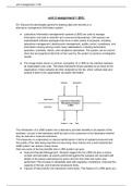
Write a MATLAB function to simulate and plot the steady-state response x(t) of an undamped
single-degree-of-freedom (SDOF) system subjected to a harmonic force F(t)=100cos(ωt).
Evaluate the system response over an excitation frequency range of ω=1 to 40 rad/s. Provide a
brief interpretation of the resulting plot. (7)
Matlab
function undamped_response()
% Parameters
m = 10; % kg
k = 4000; % N/m
F0 = 100; % N
omega_n = sqrt(k/m); % Natural frequency, rad/s
% Frequency range
omega = linspace(1, 40, 1000); % rad/s
% Steady-state amplitude (magnitude of x(t))
amplitude = F0 ./ abs(k - m * omega.^2);
% Plot
figure;
plot(omega, amplitude);
xlabel('Excitation Frequency \omega (rad/s)');
ylabel('Amplitude of x(t) (m)');
title('Steady-State Response Amplitude vs. Frequency (Undamped)' );
grid on;
hold on;
plot([omega_n omega_n], [0 max(amplitude)], 'r--'); % Resonance line
legend('Amplitude', 'Resonance');
end
, Output
Assignment 02
Due Year 2025
,Question 1 [28]
A team of mechanical engineers is tasked with analysing the dynamic behavior of a single-
degree-of-freedom (SDOF) mechanical system subjected to various forms of harmonic
excitation. The goal is to understand the system's steady-state response under different
scenarios, including undamped and damped conditions, base excitation, and rotating
unbalance. The engineers are required to simulate these cases using MATLAB and interpret the
results through appropriate plots. The mechanical system under investigation has a mass of
m=10 kg and stiffness of k=4000 N/m.
Question 1.1
Write a MATLAB function to simulate and plot the steady-state response x(t) of an undamped
single-degree-of-freedom (SDOF) system subjected to a harmonic force F(t)=100cos(ωt).
Evaluate the system response over an excitation frequency range of ω=1 to 40 rad/s. Provide a
brief interpretation of the resulting plot. (7)
Matlab
function undamped_response()
% Parameters
m = 10; % kg
k = 4000; % N/m
F0 = 100; % N
omega_n = sqrt(k/m); % Natural frequency, rad/s
% Frequency range
omega = linspace(1, 40, 1000); % rad/s
% Steady-state amplitude (magnitude of x(t))
amplitude = F0 ./ abs(k - m * omega.^2);
% Plot
figure;
plot(omega, amplitude);
xlabel('Excitation Frequency \omega (rad/s)');
ylabel('Amplitude of x(t) (m)');
title('Steady-State Response Amplitude vs. Frequency (Undamped)' );
grid on;
hold on;
plot([omega_n omega_n], [0 max(amplitude)], 'r--'); % Resonance line
legend('Amplitude', 'Resonance');
end
, Output