Solutions Manual to Romer's Advanced Macroeconomics
5th Edition Complete Solution Manual David Romer All
Chapters ||Complete A+ Guide
SOLUTIONS TO CHAPTER 1
Problem 1.1
(a) Since the growth rate of a variable equals the time derivative of its log, as shown by equation (1.10)
in the text, we can write
Ż(t) d ln Z(t) d lnX(t)Y(t)
(1) .
Z(t) dt dt
Since the log of the product of two variables equals the sum of their logs, we have
Ż(t) dln X(t) ln Y(t) d ln X(t) d ln Y(t)
(2) ,
Z(t) dt dt dt
or simply
Ż(t) Ẋ(t) Ẏ(t)
(3) .
Z(t) X(t) Y(t)
(b) Again, since the growth rate of a variable equals the time derivative of its log, we can write
Ż(t) d ln Z(t) d lnX(t) Y(t)
(4) .
Z(t) dt dt
Since the log of the ratio of two variables equals the difference in their logs, we have
Ż(t) dln X(t) ln Y(t) d ln X(t) d ln Y(t)
(5) ,
Z(t) dt dt dt
or simply
Ż(t) Ẋ(t) Ẏ(t)
(6) .
Z(t) X(t) Y(t)
(c) We have
Ż(t) d ln Z(t) d ln[X(t) ]
(7) .
Z(t) dt dt
Using the fact that ln[X(t) ] = lnX(t), we have
Ż(t) d ln X(t) d ln X(t) Ẋ (t)
(8) ,
Z(t) dt dt X(t)
where we have used the fact that is a constant.
Problem 1.2
(a) Using the information provided in the question,
the path of the growth rate of X, Ẋ(t) X(t), is Ẋ(t)
depicted in the figure at right. X(t)
© 2012 by McGraw-Hill Education. This is proprietary material solely for authorized instructor use. Not authorized for sale or distribution in any
manner. This document may not be copied, scanned, duplicated, forwarded, distributed, or posted on a website, in whole or part.
,From time 0 to time t1 , the growth rate of X is
constant and equal to a > 0. At time t1 , the growth
rate of X drops to 0. From time t1 to time t2 , the
growth rate of X rises gradually from 0 to a. Note that
we have made the assumption that Ẋ(t) X(t) rises at
a constant rate from t1 to t2 . Finally, after time t2 , the
growth rate of X is constant and equal to a again.
© 2012 by McGraw-Hill Education. This is proprietary material solely for authorized instructor use. Not authorized for sale or distribution in any
manner. This document may not be copied, scanned, duplicated, forwarded, distributed, or posted on a website, in whole or part.
,
, 1-2 Solutions to Chapter 1
(b) Note that the slope of lnX(t) plotted against time
is equal to the growth rate of X(t). That is, we know lnX(t)
d ln X(t) Ẋ (t) slope = a
dt X(t)
(See equation (1.10) in the text.) slope = a
From time 0 to time t1 the slope of lnX(t) equals
a > 0. The lnX(t) locus has an inflection point at t1 ,
when the growth rate of X(t) changes discontinuously lnX(0)
from a to 0. Between t1 and t2 , the slope of lnX(t)
rises gradually from 0 to a. After time t2 the slope of
lnX(t) is constant and equal to a > 0 again. 0 t1 t2 time
Problem 1.3
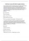
(a) The slope of the break-even investment line is
Inv/ (n + g + )k
given by (n + g + ) and thus a fall in the rate of eff lab
depreciation, , decreases the slope of the break-
even investment line. (n + g + NEW)k
The actual investment curve, sf(k) is unaffected.
sf(k)
From the figure at right we can see that the balanced-
growth-path level of capital per unit of effective
labor rises from k* to k*NEW .
k* k*NEW k
(b) Since the slope of the break-even investment
line is given by (n + g + ), a rise in the rate of Inv/ (n + gNEW + )k
technological progress, g, makes the break-even eff lab
investment line steeper.
(n + g + )k
The actual investment curve, sf(k), is unaffected.
sf(k)
From the figure at right we can see that the
balanced-growth-path level of capital per unit of
effective labor falls from k* to k*NEW .
k*NEW k* k
© 2012 by McGraw-Hill Education. This is proprietary material solely for authorized instructor use. Not authorized for sale or distribution in any
manner. This document may not be copied, scanned, duplicated, forwarded, distributed, or posted on a website, in whole or part.
5th Edition Complete Solution Manual David Romer All
Chapters ||Complete A+ Guide
SOLUTIONS TO CHAPTER 1
Problem 1.1
(a) Since the growth rate of a variable equals the time derivative of its log, as shown by equation (1.10)
in the text, we can write
Ż(t) d ln Z(t) d lnX(t)Y(t)
(1) .
Z(t) dt dt
Since the log of the product of two variables equals the sum of their logs, we have
Ż(t) dln X(t) ln Y(t) d ln X(t) d ln Y(t)
(2) ,
Z(t) dt dt dt
or simply
Ż(t) Ẋ(t) Ẏ(t)
(3) .
Z(t) X(t) Y(t)
(b) Again, since the growth rate of a variable equals the time derivative of its log, we can write
Ż(t) d ln Z(t) d lnX(t) Y(t)
(4) .
Z(t) dt dt
Since the log of the ratio of two variables equals the difference in their logs, we have
Ż(t) dln X(t) ln Y(t) d ln X(t) d ln Y(t)
(5) ,
Z(t) dt dt dt
or simply
Ż(t) Ẋ(t) Ẏ(t)
(6) .
Z(t) X(t) Y(t)
(c) We have
Ż(t) d ln Z(t) d ln[X(t) ]
(7) .
Z(t) dt dt
Using the fact that ln[X(t) ] = lnX(t), we have
Ż(t) d ln X(t) d ln X(t) Ẋ (t)
(8) ,
Z(t) dt dt X(t)
where we have used the fact that is a constant.
Problem 1.2
(a) Using the information provided in the question,
the path of the growth rate of X, Ẋ(t) X(t), is Ẋ(t)
depicted in the figure at right. X(t)
© 2012 by McGraw-Hill Education. This is proprietary material solely for authorized instructor use. Not authorized for sale or distribution in any
manner. This document may not be copied, scanned, duplicated, forwarded, distributed, or posted on a website, in whole or part.
,From time 0 to time t1 , the growth rate of X is
constant and equal to a > 0. At time t1 , the growth
rate of X drops to 0. From time t1 to time t2 , the
growth rate of X rises gradually from 0 to a. Note that
we have made the assumption that Ẋ(t) X(t) rises at
a constant rate from t1 to t2 . Finally, after time t2 , the
growth rate of X is constant and equal to a again.
© 2012 by McGraw-Hill Education. This is proprietary material solely for authorized instructor use. Not authorized for sale or distribution in any
manner. This document may not be copied, scanned, duplicated, forwarded, distributed, or posted on a website, in whole or part.
,
, 1-2 Solutions to Chapter 1
(b) Note that the slope of lnX(t) plotted against time
is equal to the growth rate of X(t). That is, we know lnX(t)
d ln X(t) Ẋ (t) slope = a
dt X(t)
(See equation (1.10) in the text.) slope = a
From time 0 to time t1 the slope of lnX(t) equals
a > 0. The lnX(t) locus has an inflection point at t1 ,
when the growth rate of X(t) changes discontinuously lnX(0)
from a to 0. Between t1 and t2 , the slope of lnX(t)
rises gradually from 0 to a. After time t2 the slope of
lnX(t) is constant and equal to a > 0 again. 0 t1 t2 time
Problem 1.3
(a) The slope of the break-even investment line is
Inv/ (n + g + )k
given by (n + g + ) and thus a fall in the rate of eff lab
depreciation, , decreases the slope of the break-
even investment line. (n + g + NEW)k
The actual investment curve, sf(k) is unaffected.
sf(k)
From the figure at right we can see that the balanced-
growth-path level of capital per unit of effective
labor rises from k* to k*NEW .
k* k*NEW k
(b) Since the slope of the break-even investment
line is given by (n + g + ), a rise in the rate of Inv/ (n + gNEW + )k
technological progress, g, makes the break-even eff lab
investment line steeper.
(n + g + )k
The actual investment curve, sf(k), is unaffected.
sf(k)
From the figure at right we can see that the
balanced-growth-path level of capital per unit of
effective labor falls from k* to k*NEW .
k*NEW k* k
© 2012 by McGraw-Hill Education. This is proprietary material solely for authorized instructor use. Not authorized for sale or distribution in any
manner. This document may not be copied, scanned, duplicated, forwarded, distributed, or posted on a website, in whole or part.