Module 2: Auto-Regressive and Moving Average Model
Module 2 Road Map
This lesson is an overview of the content covered in the second module of the Time series Course.
Course Road Map
This course roadmap displays the material covered in the course starting with the pre-requisites needed for a better and deeper
understanding of the different time series models introduced in this course. The course beings with basic concepts of time series
analysis including trend and seasonality analysis as well as an understanding of the dependence in a time series. The rest of the
course follows in presenting three main modeling approaches commonly employed in time series analysis; they are the ARMA,
GARCH and VAR models. I will provide a more detailed reference on these models next.
Course Road Map: Univariate Analysis
We will continue with modeling approaches for analyzing univariate time series; that is, analyzing one time series in isolation of any
other exogeneous factors. We will differentiate between modeling the mean or the variance; more specifically, conditional mean and
,conditional variance since they depend on past data. One set of models will be developed for the conditional mean and another for
the conditional variance.
Module 2 introduces one of the most common modeling approaches for time series analysis, specifically, the so called ARMA
models; ARMA stands for Autoregressive Moving Average. ARMA models apply to stationary processes. However, we can extend
the ARMA model to apply to non-stationary time series by applying differencing, a common approach used when a time series is
non-stationary due to trend and seasonality. The resulting model is ARIMA, which stands for Integrated ARMA. If there is also
seasonality in the time series, we can go one step further to the Seasonal ARIMA. Because the ARMA models are linear models,
again we will apply the best linear predictor to obtain predictions for future data.
ARMA Models
What will this module cover? In the first part of this module, I will cover the fundamentals of the ARMA modeling, such as the
decomposition of ARMA into the AR or Autoregressive component and the MA or Moving Average component. With that, you will
learn about dependence in a time series measured by the auto-covariance and auto-correlation under an ARMA model. Last, you
will learn about two important characteristics, causality and invertibility.
The fundamentals of ARMA modeling are the grounding of many time series models, including GARCH and VAR models.
ARMA Models (cont’d)
I will next move onto ARMA model estimation, introducing multiple methods, including methods of moments as well maximum
likelihood estimation. I will also illustrate how the autoregressive model can reduce to a linear regression model. For the fitting of an
ARMA model, we also need to perform model selection and to evaluate the model. Last, I will describe the prediction approach
using an ARMA model.
ARMA estimation and inference is used in model interpretation and evaluation hence it is important to understand those concepts.
ARMA Models (cont’d)
The basic ARMA model applies to stationary time series. What can we do if we have non-stationary time series? We can remove
the trend and seasonality and then analyze the residual process using the ARMA process. But we can also use an extension of the
ARMA model that applies to non-stationary time series called ARIMA or integrated ARMA. Further I will describe another extension
the Seasonal ARMA that extends the ARMA to seasonal time series.
Because ARMA and its extensions apply to stationary and non-stationary time series, ARMA models can be applied broadly to
many time series with various characteristics.
Data Examples using R Statistical Software
Throughout this module we will also experiment the main concepts using three data examples. In these examples, we will analyze
the daily patient volume in the emergency department in a hospital over a period of five years, focusing on the trend and seasonality
estimation as well as prediction, useful in staffing and management. A second example is the analysis of the IBM stock price; IBM
was selected to be analyzed since it has been around for more than 50 years. Last, we will explore in detail the U.S. Fuel
Consumption as proxy of energy consumption over 15 years of data. We will analyze these three data examples using the R
statistical software. We will perform exploratory data analysis using visual analytics, we will evaluate the goodness of fit and the
performance of the ARMA fit and we will use the ARMA model for predictions.
It is important to practice with real data examples because fundamentals of time series modeling are best understood by illustrating
them using data examples.
Summary:
This lesson overviewed the main topics covered in Module 2. Let’s now begin with the lessons overviewing the main concepts of
ARMA.
,2.1: Introductory Concepts and Definitions
2.1.1 Basic Concepts
In this lesson, I'll introduce one of the most useful time series models, the autoregressive moving average or ARMA model, which is
the basis of all the models introduced in this course. Hence in this lesson you will learn about the definition and fundamentals of
ARMA.
is a stochastic process in which is a set of time points usuall
or
The is a collection of random variables
that represent an un nown behavior of a phenomenon situation
process over time.
The is a set of data values observed over successive
times representing the behavior of a phenomenon situation process over
time. The are one e l t on of the stochastic time series
The term time series is also used to refer to the reali ation of such a
process observed time series .
Let's recall the definition of a time series: It is a sequence or collection of random variables with some similarity in terms of the
probability distribution, called a stochastic process. For a time series, the sequence of random variables is indexed by time and
observed sequentially over fixed time intervals. We differentiate between the stochastic time series that generates the time series,
which is called observed time series. It's important to highlight that the observed time series is one single realization from its
generating stochastic time series. This makes modeling time series quite challenging since we practically rely on one observation
although the time series may be for say 100 time points. Because we have one single realization of the stochastic time series, we
need to learn from the dependence of the time series to make inferences and predictions.
In this course, we refer to a time series as both the stochastic process from which you observe, and the realizations or observations
from that stochastic process. When we develop properties of the time series then we based them on the stochastic time series but
when we apply modeling then we do so on the observed time series.
, The of a time series
is if
for all o t end o s ste tc tte n e const nt
nce
for all o s dden e t e e c n es o c n e o nts
e const nt e n
for all A to de endence o se l
co el t on de ends on l t not on t e
Let's also review important concepts related to the property of stationarity of a times series, which will be further discussed in the
context of ARMA modeling. The autocovariance is a measure of dependence of a time series, as discussed in one of the lessons in
Module 1, which is defined by the covariance of any two variables of the stochastic process generating the time series. For example,
if we consider the time points r and s, the autocovariance of Xr and Xs is the expectation of the product of the mean centered
variables Xr and Xs as provided on the slide. Again here we are considering the stochastic time series to define stationary and
dependence! Further, we define the time series Xt to be weakly stationary if it has the following three conditions. Condition 1 is that
the time series has constant mean for all time points, meaning that there is no trend or systematic pattern in the time series.
Condition 2 is that it has a finite variance, or more specifically, has a finite second moment, meaning no sudden extreme changes or
change points. Condition 3 is that the autocovariance does not change when shifted in time. That is, the dependence between Xr
and Xs is the same as for the shifted Xr + t and Xs + t. This last condition also says that we have unconditional variance constant over
time. Note that I call it weakly stationary since the three conditions are first & second-order properties of the distribution of the
stochastic time series, referring to the mean, variance and serial correlation. As we will see later in this course, it is possible to have
a weakly stationary time series with higher moments changing over time. Thus, there is also a concept of strict stationarity reserved
for more rigorous conditions.
e e es e de endent d t
is a measure of auto dependence
in a time series assumed to depend onl on the lag between two variables in
the time series not the time points at which the are observed
is defined since it depends on the lag
and it does not depend on time.
however applies to
time series since it is used to evaluate stationarit hence we don t
now whether stationar in advance.
( e ll et n to t s n o e det l n d e ent lesson n t s od le
ded c ted solel to to de endence e s es o ARMA )
We will recall here the concept of autocovariance function, which is a measure of dependence for stationarity time series, following
from the third condition of stationarity as discussed in the previous slide. The auto-covariance function is the auto-covariance of any
two variables in a time series which will only depend on the lag between the two variables and not their exact time. We commonly
use the abbreviation ACF to refer to it.
Module 2 Road Map
This lesson is an overview of the content covered in the second module of the Time series Course.
Course Road Map
This course roadmap displays the material covered in the course starting with the pre-requisites needed for a better and deeper
understanding of the different time series models introduced in this course. The course beings with basic concepts of time series
analysis including trend and seasonality analysis as well as an understanding of the dependence in a time series. The rest of the
course follows in presenting three main modeling approaches commonly employed in time series analysis; they are the ARMA,
GARCH and VAR models. I will provide a more detailed reference on these models next.
Course Road Map: Univariate Analysis
We will continue with modeling approaches for analyzing univariate time series; that is, analyzing one time series in isolation of any
other exogeneous factors. We will differentiate between modeling the mean or the variance; more specifically, conditional mean and
,conditional variance since they depend on past data. One set of models will be developed for the conditional mean and another for
the conditional variance.
Module 2 introduces one of the most common modeling approaches for time series analysis, specifically, the so called ARMA
models; ARMA stands for Autoregressive Moving Average. ARMA models apply to stationary processes. However, we can extend
the ARMA model to apply to non-stationary time series by applying differencing, a common approach used when a time series is
non-stationary due to trend and seasonality. The resulting model is ARIMA, which stands for Integrated ARMA. If there is also
seasonality in the time series, we can go one step further to the Seasonal ARIMA. Because the ARMA models are linear models,
again we will apply the best linear predictor to obtain predictions for future data.
ARMA Models
What will this module cover? In the first part of this module, I will cover the fundamentals of the ARMA modeling, such as the
decomposition of ARMA into the AR or Autoregressive component and the MA or Moving Average component. With that, you will
learn about dependence in a time series measured by the auto-covariance and auto-correlation under an ARMA model. Last, you
will learn about two important characteristics, causality and invertibility.
The fundamentals of ARMA modeling are the grounding of many time series models, including GARCH and VAR models.
ARMA Models (cont’d)
I will next move onto ARMA model estimation, introducing multiple methods, including methods of moments as well maximum
likelihood estimation. I will also illustrate how the autoregressive model can reduce to a linear regression model. For the fitting of an
ARMA model, we also need to perform model selection and to evaluate the model. Last, I will describe the prediction approach
using an ARMA model.
ARMA estimation and inference is used in model interpretation and evaluation hence it is important to understand those concepts.
ARMA Models (cont’d)
The basic ARMA model applies to stationary time series. What can we do if we have non-stationary time series? We can remove
the trend and seasonality and then analyze the residual process using the ARMA process. But we can also use an extension of the
ARMA model that applies to non-stationary time series called ARIMA or integrated ARMA. Further I will describe another extension
the Seasonal ARMA that extends the ARMA to seasonal time series.
Because ARMA and its extensions apply to stationary and non-stationary time series, ARMA models can be applied broadly to
many time series with various characteristics.
Data Examples using R Statistical Software
Throughout this module we will also experiment the main concepts using three data examples. In these examples, we will analyze
the daily patient volume in the emergency department in a hospital over a period of five years, focusing on the trend and seasonality
estimation as well as prediction, useful in staffing and management. A second example is the analysis of the IBM stock price; IBM
was selected to be analyzed since it has been around for more than 50 years. Last, we will explore in detail the U.S. Fuel
Consumption as proxy of energy consumption over 15 years of data. We will analyze these three data examples using the R
statistical software. We will perform exploratory data analysis using visual analytics, we will evaluate the goodness of fit and the
performance of the ARMA fit and we will use the ARMA model for predictions.
It is important to practice with real data examples because fundamentals of time series modeling are best understood by illustrating
them using data examples.
Summary:
This lesson overviewed the main topics covered in Module 2. Let’s now begin with the lessons overviewing the main concepts of
ARMA.
,2.1: Introductory Concepts and Definitions
2.1.1 Basic Concepts
In this lesson, I'll introduce one of the most useful time series models, the autoregressive moving average or ARMA model, which is
the basis of all the models introduced in this course. Hence in this lesson you will learn about the definition and fundamentals of
ARMA.
is a stochastic process in which is a set of time points usuall
or
The is a collection of random variables
that represent an un nown behavior of a phenomenon situation
process over time.
The is a set of data values observed over successive
times representing the behavior of a phenomenon situation process over
time. The are one e l t on of the stochastic time series
The term time series is also used to refer to the reali ation of such a
process observed time series .
Let's recall the definition of a time series: It is a sequence or collection of random variables with some similarity in terms of the
probability distribution, called a stochastic process. For a time series, the sequence of random variables is indexed by time and
observed sequentially over fixed time intervals. We differentiate between the stochastic time series that generates the time series,
which is called observed time series. It's important to highlight that the observed time series is one single realization from its
generating stochastic time series. This makes modeling time series quite challenging since we practically rely on one observation
although the time series may be for say 100 time points. Because we have one single realization of the stochastic time series, we
need to learn from the dependence of the time series to make inferences and predictions.
In this course, we refer to a time series as both the stochastic process from which you observe, and the realizations or observations
from that stochastic process. When we develop properties of the time series then we based them on the stochastic time series but
when we apply modeling then we do so on the observed time series.
, The of a time series
is if
for all o t end o s ste tc tte n e const nt
nce
for all o s dden e t e e c n es o c n e o nts
e const nt e n
for all A to de endence o se l
co el t on de ends on l t not on t e
Let's also review important concepts related to the property of stationarity of a times series, which will be further discussed in the
context of ARMA modeling. The autocovariance is a measure of dependence of a time series, as discussed in one of the lessons in
Module 1, which is defined by the covariance of any two variables of the stochastic process generating the time series. For example,
if we consider the time points r and s, the autocovariance of Xr and Xs is the expectation of the product of the mean centered
variables Xr and Xs as provided on the slide. Again here we are considering the stochastic time series to define stationary and
dependence! Further, we define the time series Xt to be weakly stationary if it has the following three conditions. Condition 1 is that
the time series has constant mean for all time points, meaning that there is no trend or systematic pattern in the time series.
Condition 2 is that it has a finite variance, or more specifically, has a finite second moment, meaning no sudden extreme changes or
change points. Condition 3 is that the autocovariance does not change when shifted in time. That is, the dependence between Xr
and Xs is the same as for the shifted Xr + t and Xs + t. This last condition also says that we have unconditional variance constant over
time. Note that I call it weakly stationary since the three conditions are first & second-order properties of the distribution of the
stochastic time series, referring to the mean, variance and serial correlation. As we will see later in this course, it is possible to have
a weakly stationary time series with higher moments changing over time. Thus, there is also a concept of strict stationarity reserved
for more rigorous conditions.
e e es e de endent d t
is a measure of auto dependence
in a time series assumed to depend onl on the lag between two variables in
the time series not the time points at which the are observed
is defined since it depends on the lag
and it does not depend on time.
however applies to
time series since it is used to evaluate stationarit hence we don t
now whether stationar in advance.
( e ll et n to t s n o e det l n d e ent lesson n t s od le
ded c ted solel to to de endence e s es o ARMA )
We will recall here the concept of autocovariance function, which is a measure of dependence for stationarity time series, following
from the third condition of stationarity as discussed in the previous slide. The auto-covariance function is the auto-covariance of any
two variables in a time series which will only depend on the lag between the two variables and not their exact time. We commonly
use the abbreviation ACF to refer to it.