Introduction to Econometrics, 4th
Edition by James H Stock
Complete Chapter Solutions Manual
are included (Ch 1 to 19)
** Immediate Download
** Swift Response
** All Chapters included
** Empirical Solutions
** Exercises Solutions
,Table of Contents are given below
1.Economic Questions and Data
2.Review of Probability
3.Review of Statistics
4.Linear Regression with One Regressor
5.Regression with a Single Regressor: Hypothesis Tests and
Confidence Intervals
6.Linear Regression with Multiple Regressors
7.Hypothesis Tests and Confidence Intervals in Multiple Regression
8.Nonlinear Regression Functions
9.Assessing Studies Based on Multiple Regression
10.Regression with Panel Data
11.Regression with a Binary Dependent Variable
12.Instrumental Variables Regression
13.Experiments and Quasi-Experiments
14.Prediction with Many Regressors and Big Data
15.Introduction to Time Series Regression and Forecasting
16.Estimation of Dynamic Causal Effects
17.Additional Topics in Time Series Regression
18.The Theory of Linear Regression with One Regressor
19.The Theory of Multiple Regression
,Solutions Manual organized in reverse order, with the last chapter displayed first, to ensure
that all chapters are included in this document. (Complete Chapters included Ch19-1)
Solutions to End-of-Chapter Exercises: Chapter 19*
19.1. (a) The regression in the matrix form is
Y = Xb + U
with
⎛ TestScore ⎞ ⎛ 1 Income1 Income12 ⎞
⎜
1
⎟ ⎜ ⎟
⎜ TestScore2 ⎟ ⎜ 1 Income2 Income22 ⎟
Y= , X= ⎜ ⎟
⎜ ! ⎟
⎜ ⎟ ⎜ ! ! ! ⎟
⎜⎝ TestScoren ⎟⎠ ⎜⎝ 1 Incomen Incomen2 ⎟⎠
⎛ U ⎞
⎜
1
⎟ ⎛ β ⎞
0
⎜ U2 ⎟ ⎜ ⎟
U=
⎜ ! ⎟
, β = ⎜ β1 ⎟ .
⎜ ⎟ ⎜ β ⎟
⎜⎝ U n ⎟⎠ ⎝ 2 ⎠
(b) The null hypothesis is
Rb = r
versus Rb ¹ r with
R = ( 0 0 1 ) and r = 0.
The heteroskedasticity-robust F-statistic testing the null hypothesis is
-1
F = (Rβˆ - r)¢ é RΣ
ˆ R¢ù (Rβˆ - r )/q
ë βˆ û
With q = 1. Under the null hypothesis,
d
F→ Fq, ∞ .
We reject the null hypothesis if the calculated F-statistic is larger than the critical
value of the Fq ,¥ distribution at a given significance level.
, Stock/Watson - Introduction to Econometrics - 4th Edition - Answers to Exercises: Chapter 19 2
_____________________________________________________________________________________________________
19.2. (a) The sample size n = 20. We write the regression in the matrix from:
Y = Xb + U
with
⎛ Y1 ⎞ ⎛ X 2,1 ⎞
⎜ ⎟ 1 X 1,1
⎜ Y2 ⎟ ⎜ ⎟
Y=⎜ ⎟ ⎜ 1 X 1, 2 X 2, 2 ⎟
! ⎟ , X=⎜ ⎟
⎜
⎜⎝ Yn ⎟⎠ ⎜ ! ! ! ⎟
⎜ 1 X 1, n X 2, n ⎟⎠
⎝
⎛ u1 ⎞
⎜ ⎟ ⎛ β ⎞
⎜ ⎟
0
⎜ u2 ⎟
U=⎜ ⎟, β = ⎜ β1 ⎟
⎜ ! ⎟ ⎜ ⎟
⎜⎝ un ⎟⎠ ⎝ β2 ⎠
The OLS estimator the coefficient vector is
β̂ = ( X′X)−1 X′Y.
with
æ n åin=1 X 1i åin=1 X 2i ö
ç ÷
X¢X = ç åin=1 X 1i åin=1 X12i åin=1 X1i X 2i ÷ ,
ç åin=1 X 1i åin=1 X1i X 2i åin=1 X 22i ÷ø
è
and
æ åin=1 Yi ö
ç ÷
X¢Y = ç åin=1 X 1iYi ÷ .
ç åin=1 X 2iYi ÷
è ø
Note
Edition by James H Stock
Complete Chapter Solutions Manual
are included (Ch 1 to 19)
** Immediate Download
** Swift Response
** All Chapters included
** Empirical Solutions
** Exercises Solutions
,Table of Contents are given below
1.Economic Questions and Data
2.Review of Probability
3.Review of Statistics
4.Linear Regression with One Regressor
5.Regression with a Single Regressor: Hypothesis Tests and
Confidence Intervals
6.Linear Regression with Multiple Regressors
7.Hypothesis Tests and Confidence Intervals in Multiple Regression
8.Nonlinear Regression Functions
9.Assessing Studies Based on Multiple Regression
10.Regression with Panel Data
11.Regression with a Binary Dependent Variable
12.Instrumental Variables Regression
13.Experiments and Quasi-Experiments
14.Prediction with Many Regressors and Big Data
15.Introduction to Time Series Regression and Forecasting
16.Estimation of Dynamic Causal Effects
17.Additional Topics in Time Series Regression
18.The Theory of Linear Regression with One Regressor
19.The Theory of Multiple Regression
,Solutions Manual organized in reverse order, with the last chapter displayed first, to ensure
that all chapters are included in this document. (Complete Chapters included Ch19-1)
Solutions to End-of-Chapter Exercises: Chapter 19*
19.1. (a) The regression in the matrix form is
Y = Xb + U
with
⎛ TestScore ⎞ ⎛ 1 Income1 Income12 ⎞
⎜
1
⎟ ⎜ ⎟
⎜ TestScore2 ⎟ ⎜ 1 Income2 Income22 ⎟
Y= , X= ⎜ ⎟
⎜ ! ⎟
⎜ ⎟ ⎜ ! ! ! ⎟
⎜⎝ TestScoren ⎟⎠ ⎜⎝ 1 Incomen Incomen2 ⎟⎠
⎛ U ⎞
⎜
1
⎟ ⎛ β ⎞
0
⎜ U2 ⎟ ⎜ ⎟
U=
⎜ ! ⎟
, β = ⎜ β1 ⎟ .
⎜ ⎟ ⎜ β ⎟
⎜⎝ U n ⎟⎠ ⎝ 2 ⎠
(b) The null hypothesis is
Rb = r
versus Rb ¹ r with
R = ( 0 0 1 ) and r = 0.
The heteroskedasticity-robust F-statistic testing the null hypothesis is
-1
F = (Rβˆ - r)¢ é RΣ
ˆ R¢ù (Rβˆ - r )/q
ë βˆ û
With q = 1. Under the null hypothesis,
d
F→ Fq, ∞ .
We reject the null hypothesis if the calculated F-statistic is larger than the critical
value of the Fq ,¥ distribution at a given significance level.
, Stock/Watson - Introduction to Econometrics - 4th Edition - Answers to Exercises: Chapter 19 2
_____________________________________________________________________________________________________
19.2. (a) The sample size n = 20. We write the regression in the matrix from:
Y = Xb + U
with
⎛ Y1 ⎞ ⎛ X 2,1 ⎞
⎜ ⎟ 1 X 1,1
⎜ Y2 ⎟ ⎜ ⎟
Y=⎜ ⎟ ⎜ 1 X 1, 2 X 2, 2 ⎟
! ⎟ , X=⎜ ⎟
⎜
⎜⎝ Yn ⎟⎠ ⎜ ! ! ! ⎟
⎜ 1 X 1, n X 2, n ⎟⎠
⎝
⎛ u1 ⎞
⎜ ⎟ ⎛ β ⎞
⎜ ⎟
0
⎜ u2 ⎟
U=⎜ ⎟, β = ⎜ β1 ⎟
⎜ ! ⎟ ⎜ ⎟
⎜⎝ un ⎟⎠ ⎝ β2 ⎠
The OLS estimator the coefficient vector is
β̂ = ( X′X)−1 X′Y.
with
æ n åin=1 X 1i åin=1 X 2i ö
ç ÷
X¢X = ç åin=1 X 1i åin=1 X12i åin=1 X1i X 2i ÷ ,
ç åin=1 X 1i åin=1 X1i X 2i åin=1 X 22i ÷ø
è
and
æ åin=1 Yi ö
ç ÷
X¢Y = ç åin=1 X 1iYi ÷ .
ç åin=1 X 2iYi ÷
è ø
Note