

!
!
!
! Packet 7: Summarizing Quantitative Data Textbook pages: 48 – 50; 53 – 72
!
After completing this material, you should be able to:
!
! • describe the distribution of a quantitative variable by discussing its shape, center, spread, and unusual
! characteristics.
!
• calculate (using StatCrunch) measures of center and measures of spread.
!
! • apply the Empirical Rule or Chebyshev’s Rule to a distribution when discussing the standard deviation.
!
! • compare distributions using boxplots.
!
! Recall: What is a quantitative variable?
!
!
!
!
!
!
To summarize a quantitative variable, we need a new graphical display – a bar graph cannot be used. We will first look at
! histograms for graphically summarizing quantitative data. What exactly is a histogram?
!
!
!
!
!
!
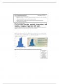
! Example: Money magazine undertook a study in 2009 to estimate the average cost for a visit to a hospital emergency
! room. A random sample of 175 emergency room visits in a certain urban area was taken, and the out-of-pocket costs
! associated with that visit were recorded. A histogram for the collected data is given below:
!
!
!
!
!
!
!
!
!
!
!
!
!
!
!
!
!
!
!
! When summarizing or describing a distribution, the following four characteristics must be discussed:
!
! 1. When asked to
!
! describe a
! 2. distribution, make
!
!
sure you address
3. these four
!
! characteristics in
! 4.
! context and in
! complete sentences.
!
, !
!
!
Packet 7: Summarizing Quantitative Data page 2
! Let’s consider each of these four characteristics individually.
!
!
Shape of the distribution
!
! When describing a distribution, the first think we should consider is what shape the distribution has. We will
!
!
consider five common shapes (shown below):
! Shape Histogram Description
!
M
!
! Measure of Center Notation Description
!
!
!
!
!
!
!
!
!
!
! The calculation of these measures, while not difficult, can be tedious. Instead of calculating these summary
! statistics by hand, we will rely on the use of StatCrunch.
!
! STA 205 Notes Buckley Fall 2018
!
!
!
! Packet 7: Summarizing Quantitative Data Textbook pages: 48 – 50; 53 – 72
!
After completing this material, you should be able to:
!
! • describe the distribution of a quantitative variable by discussing its shape, center, spread, and unusual
! characteristics.
!
• calculate (using StatCrunch) measures of center and measures of spread.
!
! • apply the Empirical Rule or Chebyshev’s Rule to a distribution when discussing the standard deviation.
!
! • compare distributions using boxplots.
!
! Recall: What is a quantitative variable?
!
!
!
!
!
!
To summarize a quantitative variable, we need a new graphical display – a bar graph cannot be used. We will first look at
! histograms for graphically summarizing quantitative data. What exactly is a histogram?
!
!
!
!
!
!
! Example: Money magazine undertook a study in 2009 to estimate the average cost for a visit to a hospital emergency
! room. A random sample of 175 emergency room visits in a certain urban area was taken, and the out-of-pocket costs
! associated with that visit were recorded. A histogram for the collected data is given below:
!
!
!
!
!
!
!
!
!
!
!
!
!
!
!
!
!
!
!
! When summarizing or describing a distribution, the following four characteristics must be discussed:
!
! 1. When asked to
!
! describe a
! 2. distribution, make
!
!
sure you address
3. these four
!
! characteristics in
! 4.
! context and in
! complete sentences.
!
, !
!
!
Packet 7: Summarizing Quantitative Data page 2
! Let’s consider each of these four characteristics individually.
!
!
Shape of the distribution
!
! When describing a distribution, the first think we should consider is what shape the distribution has. We will
!
!
consider five common shapes (shown below):
! Shape Histogram Description
!
M
!
! Measure of Center Notation Description
!
!
!
!
!
!
!
!
!
!
! The calculation of these measures, while not difficult, can be tedious. Instead of calculating these summary
! statistics by hand, we will rely on the use of StatCrunch.
!
! STA 205 Notes Buckley Fall 2018
!


