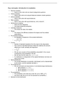
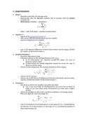
Key concepts: introduction to statistics
Nominal variables:
o Have no rank order and are closed (categorical) questions.
Ordinal variables:
o Have a rank order and unequal distances between closed questions.
Interval variables:
o Have a rank order with equal distances.
Ratio variables:
o Have a rank order with equal distances, and a natural 0.
Dichotomous variables:
o Have only two categories.
o The mean equals the proportion.
Centrality measures:
o The mode; the mean; the median.
Range:
o The range is the difference between the largest and the smallest
observations.
The standard deviation:
o An indication of dispersion of the sample distribution.
√
2
o σ = ∑ ( y i− y )
n
Z-score:
o Number of standard deviations from the mean to the observation.
o The z-score is important because it takes the relativity into account,
differences in both centrality and dispersion.
y −y
o z= ⅈ
σ
o We can use z-scores to find probabilities using table A, the z-score
corresponds to the probability in the tail.
o We can also find the value of yi: y i=( z × s ) + y
o A z-distribution is independent of the original distribution and does not
have to be normal.
Normal distribution:
o The normal distribution is symmetric, bell-shaped, and is characterised
by the mean μ and the standard deviation σ .
The empirical rule :
o We can summarise all observations in normal/bell-shaped distributions:
68% between y−s∧ y + s.
95.4% between y−2 s∧ y+ 2 s.
99.7% between y−3 s∧ y +3 s .
The probability p:
o The probability is the total area under the curve (100%, p=1).
o Any area under the curve can be expressed as probability p.
Standard normal distribution:
, o A theoretical distribution that is perfectly symmetrical and bell-shaped
with specific properties: μ=0∧σ=1.
Point estimation:
o The “best guess” of the sample statistic.
o Can vary across different samples.
Interval estimation:
o An interval of which we are quite certain that it will contain the actual
population value.
Margin of error:
o To construct a confidence interval, we subtract and add from the point
estimate a z-/t-score multiplied with the standard error.
Sample distribution:
o The known distribution of one variable in the centre.
Sampling distribution:
o A theoretical distribution of a sample statistic, that is normally
distributed and provides us with a standard error, that we in turn can
use to calculate a confidence interval.
o We cannot “get”/calculate a sampling distribution.
o Irrespective of the distribution of the variable in the population, the
sampling distribution of a statistic will be normal.
Sample statistic:
o Things we can calculate from a sample ( μ/ π ).
Central limit theorem:
o When the sample is large enough (n ≥ 30), the sampling distribution of µ
and π will follow a normal distribution.
o You can only calculate the standard error when the central limit
theorem holds.
Standard error:
o The dispersion of the sampling distribution tells us how much our point
estimate would vary between different samples, this gives us the
standard error.
o The standard deviation of the sampling distribution.
o Standard error for a proportion: se=
σ
√ π (1−π )
n
o Standard error for a mean: se=
√n
Confidence intervals:
o The confidence interval is the interval of which we are quite certain that
it contains the population mean.
o CI = ^μ∨ π^ ±( z∨t × se )
Confidence level:
o 90% z = 1.65
o 95% z = 1.96
o 99% z = 2.58
o The confidence level should be decided upfront.

