LES 3
Formal Specification and Variable Transformations (H7)
Interpretation of a coefficient?
A change in X results in a change in Y =b
An (infinitesimal) change in X leads to ??? change in Y
What is a ‘change’?
Depends on the units in which the variables were measured
Consequently, the interpretation of coefficients changes with respect to
these unit scales
metre ↔ kilometre
kilogram ↔ ton
euro ↔ 1000 euro ↔ million euro
Etc.
Impact of units
:
Since the slope coefficient β1 is marginal change in units, we need to use the right
units:
E.g. Y (in million €) and X1 (in thousand €) β1 is the impact of X1 on Y,
measured in thousand € (million/thousand) dus ook in duizend uitgedrukt
E.g. Y (in million €) and X2 (in million residents) β2 is the impact of X2 on
Y, measured in € per resident (million/million)
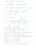
Example
Impact of walking distance on (kilo)calories burnt
Walking distance may be measured in km in meters
1
, kcal=β 0+ β1 WD
WD in km: kcal=15+50 WD
50 kcal per additional km
6 km walking: 315 kcal burnt
coefficients
9 km walking: 465 kcal burnt
differ, but
WD in meters: kcal=15+0.05 WD
interpretation
0.05 kcal per additional meter (=50kcal/km)
is identical
6000 m walking: 315 kcal burnt
9000 m walking: 465 kcal burnt
Example Gross Private Domestic Investment (GPDI) and Gross Domestic Product (GDP)
4 identical results !
(coefficients differ, but
interpretation is identical)
2
, Removing the unit scale: Standardized coefficients
Rescaling variables (op dezelfde eenheid)
All standardized variables are measured in the same unit, namely: ‘standard
deviations (away) from the mean’
Advantage
Different units of measurement are rescaled into standard deviations
Assess relative weight of impact of different variables
Example: Child mortality
CM = Child mortality, the number of deaths of children under age 5 in a year per
1000 live births.
FLRP = Female literacy rate, percent.
PGNP = per capita GNP in 1980.
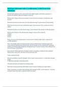
. reg cm flrp pgnp, beta
Bèta: houdt rekening met
Source SS df MS Number of obs = 64
F(2, 61) = 73.83 dezelfde eenheden
Model 257362.373 2 128681.187 Prob > F = 0.0000
Residual 106315.627 61 1742.87913 R-squared = 0.7077
Adj R-squared = 0.6981 Voordeel: coeff. knn we met
Total 363678 63 5772.66667 Root MSE = 41.748
elkaar vergelijken
cm Coef. Std. Err. t P>|t| Beta
Interpretatie: FLRP stijgt met
flrp -2.231586 .2099472 -10.63 0.000 -.7638884
pgnp -.0056466 .0020033 -2.82 0.006 -.2025703 1 eenheid dan daalt CM (Y)
_cons 263.6416 11.59318 22.74 0.000 . met 0,76 SD
Transforming our variables: Logarithmic transformations
Formal Specification of our Model
Specifications often appear to be non-linear. ( OLS: verbanden die we knn
lineairariseren)
Sometimes/often they can be ‘transformed’ into linear forms.
linearization
3
Formal Specification and Variable Transformations (H7)
Interpretation of a coefficient?
A change in X results in a change in Y =b
An (infinitesimal) change in X leads to ??? change in Y
What is a ‘change’?
Depends on the units in which the variables were measured
Consequently, the interpretation of coefficients changes with respect to
these unit scales
metre ↔ kilometre
kilogram ↔ ton
euro ↔ 1000 euro ↔ million euro
Etc.
Impact of units
:
Since the slope coefficient β1 is marginal change in units, we need to use the right
units:
E.g. Y (in million €) and X1 (in thousand €) β1 is the impact of X1 on Y,
measured in thousand € (million/thousand) dus ook in duizend uitgedrukt
E.g. Y (in million €) and X2 (in million residents) β2 is the impact of X2 on
Y, measured in € per resident (million/million)
Example
Impact of walking distance on (kilo)calories burnt
Walking distance may be measured in km in meters
1
, kcal=β 0+ β1 WD
WD in km: kcal=15+50 WD
50 kcal per additional km
6 km walking: 315 kcal burnt
coefficients
9 km walking: 465 kcal burnt
differ, but
WD in meters: kcal=15+0.05 WD
interpretation
0.05 kcal per additional meter (=50kcal/km)
is identical
6000 m walking: 315 kcal burnt
9000 m walking: 465 kcal burnt
Example Gross Private Domestic Investment (GPDI) and Gross Domestic Product (GDP)
4 identical results !
(coefficients differ, but
interpretation is identical)
2
, Removing the unit scale: Standardized coefficients
Rescaling variables (op dezelfde eenheid)
All standardized variables are measured in the same unit, namely: ‘standard
deviations (away) from the mean’
Advantage
Different units of measurement are rescaled into standard deviations
Assess relative weight of impact of different variables
Example: Child mortality
CM = Child mortality, the number of deaths of children under age 5 in a year per
1000 live births.
FLRP = Female literacy rate, percent.
PGNP = per capita GNP in 1980.
. reg cm flrp pgnp, beta
Bèta: houdt rekening met
Source SS df MS Number of obs = 64
F(2, 61) = 73.83 dezelfde eenheden
Model 257362.373 2 128681.187 Prob > F = 0.0000
Residual 106315.627 61 1742.87913 R-squared = 0.7077
Adj R-squared = 0.6981 Voordeel: coeff. knn we met
Total 363678 63 5772.66667 Root MSE = 41.748
elkaar vergelijken
cm Coef. Std. Err. t P>|t| Beta
Interpretatie: FLRP stijgt met
flrp -2.231586 .2099472 -10.63 0.000 -.7638884
pgnp -.0056466 .0020033 -2.82 0.006 -.2025703 1 eenheid dan daalt CM (Y)
_cons 263.6416 11.59318 22.74 0.000 . met 0,76 SD
Transforming our variables: Logarithmic transformations
Formal Specification of our Model
Specifications often appear to be non-linear. ( OLS: verbanden die we knn
lineairariseren)
Sometimes/often they can be ‘transformed’ into linear forms.
linearization
3