,TABLE
TableOF
ofCONTENTS
Contents
PRERIQUISTIES AND COGNITIVE LEVELS
Differentiation from First Principles
1.(from CAPS curriculum)
Differentiation from First Principles
• The rate of change at a point
• Determining the derivative using first principles
Differentiation Rules
2. Differentiation Rules
• Laws of Differentiation & Notation
• Tangent to a curve
Cubic Functions
3. Cubic Functions
• Factorizing a Cubic Function
• Parts of a Cubic Function
o Turning Point
o Concavity
o Inflection Point
• Finding the equation of a cubic function
o 𝑥-intercepts given
o Turning points given
o Derivative given
Applications of Calculus
4. Applications of Calculus
• Optimization (minima & maxima)
Exam Practice
5. Exam Practice
2
,DIFFERENTIATION USING FIRST PRINCIPLES
The rate of change at a point
The derivative of a function simply means the rate of change at a certain point on our
function.
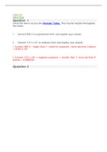
Let’s assume we have a random function, 𝑓(𝑥), as depicted below:
𝒚 𝒇(𝒙)
𝐴(𝑥; 𝑓 𝑥 )
𝒙
On this function, we have a certain point called A (as seen above). If we want to know the
rate of change at point A, we first need to find another point on our function called B. We
then would need to calculate average gradient between point A and B.
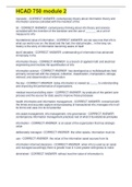
Note: the coordinates of point A is (𝑥 ; 𝑓 𝑥 ). The 𝑥-value for B is at certain distance (𝒉) from
the 𝑥-value of point A, thus its 𝑥-coordinate for point B is 𝑥 + ℎ. The 𝑦-value for point B is the
value of the function at 𝑥 + ℎ thus the coordinates of point B is (𝑥 + ℎ ; 𝑓(𝑥 + ℎ)).
Plotting both points A and B we get:
𝒚 𝒇(𝒙)
𝐵(𝑥 + ℎ; 𝑓 𝑥 + ℎ )
𝐴(𝑥; 𝑓 𝑥 )
𝒙
Distance(𝒉)
3
, Now that we have plotted our two points A and B, we can determine the average gradient
using this formula:
𝑦𝐵 − 𝑦𝐴
𝑚𝑎𝑣𝑒 =
𝑥𝐵 − 𝑥𝐴
Substituting our coordinates for A and B we get:
𝑓 𝑥 + ℎ − 𝑓(𝑥)
𝑚𝑎𝑣𝑒 =
𝑥+ℎ −𝑥
Simplifying we get:
𝒇 𝒙 + 𝒉 − 𝒇(𝒙)
𝒎𝒂𝒗𝒆 =
𝒉
This equation tells us the average rate of change of our function between any two points.
The average rate of change can be represented as the gradient of a straight line which passes
through points A and B as shown below:
𝒚 𝒇(𝒙)
𝑩
𝑨
𝒙
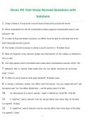
If we want to know what the rate of change at point A is, we simply decrease the distance, ℎ,
between our two points and continue to do so until our distance gets infinitely closer to zero.
At this point our different points will be so close together, that the straight line that passes
through them will become a tangent to the function 𝑓(𝑥).
𝒚
𝒇(𝒙)
Note: the distance between
points A and B NEVER
reaches zero, it just gets
closer and closer to zero
𝑨 forever ... that’s how cool
infinity is!
𝒙
4
TableOF
ofCONTENTS
Contents
PRERIQUISTIES AND COGNITIVE LEVELS
Differentiation from First Principles
1.(from CAPS curriculum)
Differentiation from First Principles
• The rate of change at a point
• Determining the derivative using first principles
Differentiation Rules
2. Differentiation Rules
• Laws of Differentiation & Notation
• Tangent to a curve
Cubic Functions
3. Cubic Functions
• Factorizing a Cubic Function
• Parts of a Cubic Function
o Turning Point
o Concavity
o Inflection Point
• Finding the equation of a cubic function
o 𝑥-intercepts given
o Turning points given
o Derivative given
Applications of Calculus
4. Applications of Calculus
• Optimization (minima & maxima)
Exam Practice
5. Exam Practice
2
,DIFFERENTIATION USING FIRST PRINCIPLES
The rate of change at a point
The derivative of a function simply means the rate of change at a certain point on our
function.
Let’s assume we have a random function, 𝑓(𝑥), as depicted below:
𝒚 𝒇(𝒙)
𝐴(𝑥; 𝑓 𝑥 )
𝒙
On this function, we have a certain point called A (as seen above). If we want to know the
rate of change at point A, we first need to find another point on our function called B. We
then would need to calculate average gradient between point A and B.
Note: the coordinates of point A is (𝑥 ; 𝑓 𝑥 ). The 𝑥-value for B is at certain distance (𝒉) from
the 𝑥-value of point A, thus its 𝑥-coordinate for point B is 𝑥 + ℎ. The 𝑦-value for point B is the
value of the function at 𝑥 + ℎ thus the coordinates of point B is (𝑥 + ℎ ; 𝑓(𝑥 + ℎ)).
Plotting both points A and B we get:
𝒚 𝒇(𝒙)
𝐵(𝑥 + ℎ; 𝑓 𝑥 + ℎ )
𝐴(𝑥; 𝑓 𝑥 )
𝒙
Distance(𝒉)
3
, Now that we have plotted our two points A and B, we can determine the average gradient
using this formula:
𝑦𝐵 − 𝑦𝐴
𝑚𝑎𝑣𝑒 =
𝑥𝐵 − 𝑥𝐴
Substituting our coordinates for A and B we get:
𝑓 𝑥 + ℎ − 𝑓(𝑥)
𝑚𝑎𝑣𝑒 =
𝑥+ℎ −𝑥
Simplifying we get:
𝒇 𝒙 + 𝒉 − 𝒇(𝒙)
𝒎𝒂𝒗𝒆 =
𝒉
This equation tells us the average rate of change of our function between any two points.
The average rate of change can be represented as the gradient of a straight line which passes
through points A and B as shown below:
𝒚 𝒇(𝒙)
𝑩
𝑨
𝒙
If we want to know what the rate of change at point A is, we simply decrease the distance, ℎ,
between our two points and continue to do so until our distance gets infinitely closer to zero.
At this point our different points will be so close together, that the straight line that passes
through them will become a tangent to the function 𝑓(𝑥).
𝒚
𝒇(𝒙)
Note: the distance between
points A and B NEVER
reaches zero, it just gets
closer and closer to zero
𝑨 forever ... that’s how cool
infinity is!
𝒙
4