ISYE 6402 Midterm 2 (V2) Questions and 100% Correct Answers 2026/27 Latest-
Georgia Institute Of Technology.
Background
For this midterm exam, you will analyze vehicular collision data for the New York City borough of Manhattan. The data records the number of
collisions involving motor vehicles in Manhattan each week from the beginning of 2013 to the end of 2021. Columns yr and wk designate the year
and week number during which each data point was recorded, respectively, while the collisions column records the number of collisions during that
week.
library(zoo)
library(lubridate)
library(mgcv)
library(TSA)
library(dynlm)
library(rugarch)
library(tseries)
library(fGarch)
Instructions on reading the data
To read the data in R , save the file in your working directory (make sure you have changed the directory if different from the R working directory)
and read the data using the R function read.csv()
#Read in data, split into full and abridged data
colls<-read.csv("Midterm 2 Data.csv")
Training & Testing Data
For this data analysis, you will divide the data as follows.
Pre-pandemic analysis: The training data will consists of years 2013-2018 and the year 2019 excluding the last 8 weeks of the year. The last 8
weeks of 2019 will will then be the testing data. The predictions in this analysis will be 4-week rolling predictions; that is first obtain the predictions
of the first four weeks out of the eight weeks of training data, then the training data are updated to include these four weeks so that the last four
weeks of 2019 to be predicted.
Pandemic analysis: The training data will consists of years 2013-2020 and the year 2021 excluding the last 8 weeks of this year. The last 8 weeks
of 2021 will then be the testing data. The predictions in this analysis will be 4-week rolling predictions; that is first obtain the predictions of the first
four weeks out of the eight weeks of training data, then the training data are updated to include these four weeks so that the last four weeks of
2021 to be predicted. This analysis will be done with and without the 2020 pandemic year.
Part 1: Exploratory Data Analysis of the Entire Time Series
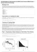
1a. Plot the Time Series and the ACF plots for the entire data. Comment on the stationarity of the data, as well as any features of note.
colls.ts<-ts(colls$collisions,start=2013,freq=52)
par(mfrow=c(1,2))
plot(colls.ts,ylab="Collisions",main="Collisions-Time Series")
acf(colls.ts,lag.max=52*4,main="Collisions-ACF")
,Response: Question 1a
The time series plot of the data clearly exhibits a non-constant mean, as well as fluctuations in variance, which decreases notably from the
beginning of the COVID-19 pandemic onward. The ACF plot confirms the presence of a trend in the data. The data is not stationary.
1b. Plot the Time Series and the ACF plots for the differenced data. Compare these plots with the plots that you produced in question 1(a) in terms
of the assumptions of stationarity.
colls.diff.ts<-diff(colls.ts)
par(mfrow=c(1,2))
plot(colls.diff.ts,ylab="Collisions (Differenced)",main="Collisions (Differenced)-Time Series")
acf(colls.diff.ts,lag.max=52*4,main="Collisions (Differenced)-ACF")
Response: Question 1b
Differencing the data has removed the trend, but has made the non-constant nature of the variance in the data even more apparent. The ACF plot
of the differenced data seems to indicate the presence of possible seasonality in the data, with significant spikes at the scaled lags. Because of the
clear presence of heteroskedasticity and the possible presence of seasonality in the differenced data, we cannot conclude that the differenced data
is stationary.
1c. Comment on the appropriateness of using both ARIMA and ARMA-GARCH methods to model the data based on the data features that you
observed in 1(a) and 1(b). What other data features (if any) should be considered when selecting an appropriate method for modeling the collision
data?
Response: Question 1c
ARIMA modeling would likely be a poor option to use to model the data due to the heteroskedasticity in the data. ARMA-GARCH modeling would
likely prove a better method for modeling the data. Given our observations in 1(b), it could also prove helpful to choose a method to model the data
which includes a seasonal component.
Part 2: Model Fitting: Pre-pandemic Data Analysis
2a. Fit a seasonality model on the training data using the ANOVA approach. Derive the residuals of the seasonality model. Use the iterative
approach to choose the optimal orders for an ARIMA model fit to the residual training data, using max (p,d,q) of (4,1,4) and selecting with the AIC
score. Fit the model with the selected ARIMA order to the residual training data and call this model model1. Indicate the orders you selected and
comment on the statistical significance of the model coefficients.
, pre<-colls[colls$yr < 2020,]
pre.ts<-ts(pre$collisions,start=2013,freq=52)
l<-length(pre.ts)
pre.seas<-lm(pre.ts~season(pre.ts))
pre.resids<-ts(pre.seas$residuals)
pre.resids.train<-pre.resids[1:(l-8)]
pre.resids.test<-pre.resids[(l-7):l]
#Fit ARIMA model to residuals of seasonal model
test_modelA <- function(p,d,q){
mod = arima(pre.resids.train, order=c(p,d,q),method="ML")
current.aic = AIC(mod)
df = data.frame(p,d,q,current.aic)
names(df) <- c("p","d","q","AIC")
#print(paste(p,d,q,current.aic,sep=" "))
return(df)
}
orders = data.frame(Inf,Inf,Inf,Inf)
names(orders) <- c("p","d","q","AIC")
for (p in 0:4){
for (d in 0:1){
for (q in 0:4) {
possibleError <- tryCatch(
orders<-rbind(orders,test_modelA(p,d,q)),
error=function(e) e
)
if(inherits(possibleError, "error")) next
}
}
}
orders <- orders[order(-orders$AIC),]
tail(orders,5)
## p d q AIC
## 10 0 1 3 3765.690
## 28 2 1 1 3765.334
## 51 4 1 4 3764.605
## 40 3 1 3 3764.189
## 31 2 1 4 3762.134
model1<-arima(pre.resids.train, order=c(2,1,4),method="ML")
model1
##
## Call:
## arima(x = pre.resids.train, order = c(2, 1, 4), method = "ML")
##
## Coefficients:
## ar1 ar2 ma1 ma2 ma3 ma4
## -1.6367 -0.9022 0.7566 -0.4628 -0.6172 0.2027
## s.e. 0.0293 0.0281 0.0614 0.0596 0.0632 0.0597
##
## sigma^2 estimated as 2218: log likelihood = -1874.07, aic = 3760.13
cat("\nModel1 p-values:\n")
##
## Model1 p-values:
model1.coefs <-as.numeric(model1$coef)/as.numeric(sqrt(diag(model1$var.coef)))
model1.pvals <- 2 * (1 - pnorm(abs(model1.coefs)))
model1.pvals
## [1] 0.000000e+00 0.000000e+00 0.000000e+00 8.437695e-15 0.000000e+00
## [6] 6.787945e-04
Response: Question 2a
Orders (2,1,4) have the lowest AIC value. All the coefficients of the ARIMA (2,1,4) model fit to the residual training data are statistically significant.
Georgia Institute Of Technology.
Background
For this midterm exam, you will analyze vehicular collision data for the New York City borough of Manhattan. The data records the number of
collisions involving motor vehicles in Manhattan each week from the beginning of 2013 to the end of 2021. Columns yr and wk designate the year
and week number during which each data point was recorded, respectively, while the collisions column records the number of collisions during that
week.
library(zoo)
library(lubridate)
library(mgcv)
library(TSA)
library(dynlm)
library(rugarch)
library(tseries)
library(fGarch)
Instructions on reading the data
To read the data in R , save the file in your working directory (make sure you have changed the directory if different from the R working directory)
and read the data using the R function read.csv()
#Read in data, split into full and abridged data
colls<-read.csv("Midterm 2 Data.csv")
Training & Testing Data
For this data analysis, you will divide the data as follows.
Pre-pandemic analysis: The training data will consists of years 2013-2018 and the year 2019 excluding the last 8 weeks of the year. The last 8
weeks of 2019 will will then be the testing data. The predictions in this analysis will be 4-week rolling predictions; that is first obtain the predictions
of the first four weeks out of the eight weeks of training data, then the training data are updated to include these four weeks so that the last four
weeks of 2019 to be predicted.
Pandemic analysis: The training data will consists of years 2013-2020 and the year 2021 excluding the last 8 weeks of this year. The last 8 weeks
of 2021 will then be the testing data. The predictions in this analysis will be 4-week rolling predictions; that is first obtain the predictions of the first
four weeks out of the eight weeks of training data, then the training data are updated to include these four weeks so that the last four weeks of
2021 to be predicted. This analysis will be done with and without the 2020 pandemic year.
Part 1: Exploratory Data Analysis of the Entire Time Series
1a. Plot the Time Series and the ACF plots for the entire data. Comment on the stationarity of the data, as well as any features of note.
colls.ts<-ts(colls$collisions,start=2013,freq=52)
par(mfrow=c(1,2))
plot(colls.ts,ylab="Collisions",main="Collisions-Time Series")
acf(colls.ts,lag.max=52*4,main="Collisions-ACF")
,Response: Question 1a
The time series plot of the data clearly exhibits a non-constant mean, as well as fluctuations in variance, which decreases notably from the
beginning of the COVID-19 pandemic onward. The ACF plot confirms the presence of a trend in the data. The data is not stationary.
1b. Plot the Time Series and the ACF plots for the differenced data. Compare these plots with the plots that you produced in question 1(a) in terms
of the assumptions of stationarity.
colls.diff.ts<-diff(colls.ts)
par(mfrow=c(1,2))
plot(colls.diff.ts,ylab="Collisions (Differenced)",main="Collisions (Differenced)-Time Series")
acf(colls.diff.ts,lag.max=52*4,main="Collisions (Differenced)-ACF")
Response: Question 1b
Differencing the data has removed the trend, but has made the non-constant nature of the variance in the data even more apparent. The ACF plot
of the differenced data seems to indicate the presence of possible seasonality in the data, with significant spikes at the scaled lags. Because of the
clear presence of heteroskedasticity and the possible presence of seasonality in the differenced data, we cannot conclude that the differenced data
is stationary.
1c. Comment on the appropriateness of using both ARIMA and ARMA-GARCH methods to model the data based on the data features that you
observed in 1(a) and 1(b). What other data features (if any) should be considered when selecting an appropriate method for modeling the collision
data?
Response: Question 1c
ARIMA modeling would likely be a poor option to use to model the data due to the heteroskedasticity in the data. ARMA-GARCH modeling would
likely prove a better method for modeling the data. Given our observations in 1(b), it could also prove helpful to choose a method to model the data
which includes a seasonal component.
Part 2: Model Fitting: Pre-pandemic Data Analysis
2a. Fit a seasonality model on the training data using the ANOVA approach. Derive the residuals of the seasonality model. Use the iterative
approach to choose the optimal orders for an ARIMA model fit to the residual training data, using max (p,d,q) of (4,1,4) and selecting with the AIC
score. Fit the model with the selected ARIMA order to the residual training data and call this model model1. Indicate the orders you selected and
comment on the statistical significance of the model coefficients.
, pre<-colls[colls$yr < 2020,]
pre.ts<-ts(pre$collisions,start=2013,freq=52)
l<-length(pre.ts)
pre.seas<-lm(pre.ts~season(pre.ts))
pre.resids<-ts(pre.seas$residuals)
pre.resids.train<-pre.resids[1:(l-8)]
pre.resids.test<-pre.resids[(l-7):l]
#Fit ARIMA model to residuals of seasonal model
test_modelA <- function(p,d,q){
mod = arima(pre.resids.train, order=c(p,d,q),method="ML")
current.aic = AIC(mod)
df = data.frame(p,d,q,current.aic)
names(df) <- c("p","d","q","AIC")
#print(paste(p,d,q,current.aic,sep=" "))
return(df)
}
orders = data.frame(Inf,Inf,Inf,Inf)
names(orders) <- c("p","d","q","AIC")
for (p in 0:4){
for (d in 0:1){
for (q in 0:4) {
possibleError <- tryCatch(
orders<-rbind(orders,test_modelA(p,d,q)),
error=function(e) e
)
if(inherits(possibleError, "error")) next
}
}
}
orders <- orders[order(-orders$AIC),]
tail(orders,5)
## p d q AIC
## 10 0 1 3 3765.690
## 28 2 1 1 3765.334
## 51 4 1 4 3764.605
## 40 3 1 3 3764.189
## 31 2 1 4 3762.134
model1<-arima(pre.resids.train, order=c(2,1,4),method="ML")
model1
##
## Call:
## arima(x = pre.resids.train, order = c(2, 1, 4), method = "ML")
##
## Coefficients:
## ar1 ar2 ma1 ma2 ma3 ma4
## -1.6367 -0.9022 0.7566 -0.4628 -0.6172 0.2027
## s.e. 0.0293 0.0281 0.0614 0.0596 0.0632 0.0597
##
## sigma^2 estimated as 2218: log likelihood = -1874.07, aic = 3760.13
cat("\nModel1 p-values:\n")
##
## Model1 p-values:
model1.coefs <-as.numeric(model1$coef)/as.numeric(sqrt(diag(model1$var.coef)))
model1.pvals <- 2 * (1 - pnorm(abs(model1.coefs)))
model1.pvals
## [1] 0.000000e+00 0.000000e+00 0.000000e+00 8.437695e-15 0.000000e+00
## [6] 6.787945e-04
Response: Question 2a
Orders (2,1,4) have the lowest AIC value. All the coefficients of the ARIMA (2,1,4) model fit to the residual training data are statistically significant.