ISYE 6402 Midterm 2 Questions and 100% Correct Answers 2026/27 Latest- Georgia
Institute Of Technology.
Background
For this midterm exam, you will analyze daily bikeshare trip data for the city of Austin, Texas. The data records the number of unique daily trips
taken by bikeshare users in the city from the beginning of 2019 to the end of June 2022. Columns ‘date’ and ‘trips’ record the date and the number
of bikeshare trips taken on the recorded date, respectively.
library(zoo)
library(lubridate)
library(mgcv)
library(TSA)
library(dynlm)
library(rugarch)
Instructions on reading the data
To read the data in R , save the file in your working directory (make sure you have changed the directory if different from the R working directory)
and read the data using the R function read.csv()
bike<-read.csv("Midterm 2 Data.csv")
Part 1: Exploratory Data Analysis
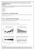
1a. Plot the time series and ACF plots for both the original and first-order differenced data. Comment on the features of the original and
differenced data. Which (if any) assumptions of stationarity are violated?
bike.ts<-ts(bike$trips,frequency = 365,start=2019)
par(mfrow=c(2,2))
plot(bike.ts,main="Austin Bikeshare Daily Trips",ylab="Trips")
acf(bike.ts,lag.max=100,main="Austin Bikeshare Daily Trips-ACF")
plot(diff(bike.ts),main="Austin Bikeshare Daily Trips (Differenced)",ylab="Trips (Differenced)")
acf(diff(bike.ts),lag.max=100,main="Austin Bikeshare Daily Trips (Differenced)-ACF")
Response: Question 1a
The time series plot of the original data shows that the data exhibits clear heteroskedasticity and has a non-constant mean. The ACF plot of the
original data shows slowly-decaying lags which also exhibit a rising and falling pattern that repeats every seventh lag, which is evidence of the
presence of both a trend and weekly seasonality in the data. Taking the first-order difference of the data removes the trend in the data; however,
, when differenced, the data’s heteroskedasticity becomes even more pronounced, and the weekly seasonality in the data still remains (as shown by
the cyclical pattern in the ACF plot of the differenced data). Neither the original nor the first-differenced data are stationary.
1b. Perform a log transformation on the original data. Plot the time series and ACF plots for both the regular and first-order differenced log-
transformed data. Evaluate the stationarity of the log-transformed data graphically. How does the stationarity of the log-transformed data compare
to that of the original data?
bike.ts.log<-ts(log(bike$trips),start=2019,frequency = 365)
par(mfrow=c(2,2))
plot(bike.ts.log,main="Log of Austin Bikeshare Daily Trips",ylab="Log Trips")
acf(bike.ts.log,lag.max = 100,main="Log of Austin Bikeshare Daily Trips-ACF")
plot(diff(bike.ts.log),main="Log of Austin Bikeshare Daily Trips (Differenced)",ylab="Log Trips (Differenced)")
acf(diff(bike.ts.log),lag.max = 100,main="Log of Austin Bikeshare Daily Trips (Differenced)-ACF")
Response: Question 1b
The log-transformed data still exhibits a non-constant mean, along with overt seasonality. Heteroskedasticity is still present in the log-transformed
data, but appears less pronounced than in the original data. The log-transformed data contains several conspicuous outliers, which are less
apparent in the original data.
1c. Based on the plots that you created in 1(a) and 1(b) and what you have learned about time series forecasting, which method do you think
would work better for modeling this data: ARIMA or ARMA-GARCH? What advantages and disadvantages might there be to modeling the log-
transformed data rather than the original data?
Response: Question 1c
Modeling the data using the ARMA-GARCH method would likely yield better forecasts due to the overt heteroskedasticity present in the data.
Applying a log transformation to the data before fitting time-series models could make the data easier to model accurately using methods which do
not account for heteroskedasticity, such as ARIMA; however, transforming the data does not completely remove the data’s heteroskedasticity, and
yields significant outliers in the data which could negatively influence model fit.
Part 2: Model Fitting: Original Data
2a. Divide both the original and the first-order differenced untransformed time series into training and test datasets, designating the last two weeks
(14 days) as the test datasets and the rest of the data as the training datasets. Fit the following models to the indicated training datasets:
ARIMA(2,1,3) on the original data, with seasonal orders (1,0,1) to model weekly seasonality
ARMA-GARCH(3,4)x(1,1) on the differenced data
Print the summary for both models.
Institute Of Technology.
Background
For this midterm exam, you will analyze daily bikeshare trip data for the city of Austin, Texas. The data records the number of unique daily trips
taken by bikeshare users in the city from the beginning of 2019 to the end of June 2022. Columns ‘date’ and ‘trips’ record the date and the number
of bikeshare trips taken on the recorded date, respectively.
library(zoo)
library(lubridate)
library(mgcv)
library(TSA)
library(dynlm)
library(rugarch)
Instructions on reading the data
To read the data in R , save the file in your working directory (make sure you have changed the directory if different from the R working directory)
and read the data using the R function read.csv()
bike<-read.csv("Midterm 2 Data.csv")
Part 1: Exploratory Data Analysis
1a. Plot the time series and ACF plots for both the original and first-order differenced data. Comment on the features of the original and
differenced data. Which (if any) assumptions of stationarity are violated?
bike.ts<-ts(bike$trips,frequency = 365,start=2019)
par(mfrow=c(2,2))
plot(bike.ts,main="Austin Bikeshare Daily Trips",ylab="Trips")
acf(bike.ts,lag.max=100,main="Austin Bikeshare Daily Trips-ACF")
plot(diff(bike.ts),main="Austin Bikeshare Daily Trips (Differenced)",ylab="Trips (Differenced)")
acf(diff(bike.ts),lag.max=100,main="Austin Bikeshare Daily Trips (Differenced)-ACF")
Response: Question 1a
The time series plot of the original data shows that the data exhibits clear heteroskedasticity and has a non-constant mean. The ACF plot of the
original data shows slowly-decaying lags which also exhibit a rising and falling pattern that repeats every seventh lag, which is evidence of the
presence of both a trend and weekly seasonality in the data. Taking the first-order difference of the data removes the trend in the data; however,
, when differenced, the data’s heteroskedasticity becomes even more pronounced, and the weekly seasonality in the data still remains (as shown by
the cyclical pattern in the ACF plot of the differenced data). Neither the original nor the first-differenced data are stationary.
1b. Perform a log transformation on the original data. Plot the time series and ACF plots for both the regular and first-order differenced log-
transformed data. Evaluate the stationarity of the log-transformed data graphically. How does the stationarity of the log-transformed data compare
to that of the original data?
bike.ts.log<-ts(log(bike$trips),start=2019,frequency = 365)
par(mfrow=c(2,2))
plot(bike.ts.log,main="Log of Austin Bikeshare Daily Trips",ylab="Log Trips")
acf(bike.ts.log,lag.max = 100,main="Log of Austin Bikeshare Daily Trips-ACF")
plot(diff(bike.ts.log),main="Log of Austin Bikeshare Daily Trips (Differenced)",ylab="Log Trips (Differenced)")
acf(diff(bike.ts.log),lag.max = 100,main="Log of Austin Bikeshare Daily Trips (Differenced)-ACF")
Response: Question 1b
The log-transformed data still exhibits a non-constant mean, along with overt seasonality. Heteroskedasticity is still present in the log-transformed
data, but appears less pronounced than in the original data. The log-transformed data contains several conspicuous outliers, which are less
apparent in the original data.
1c. Based on the plots that you created in 1(a) and 1(b) and what you have learned about time series forecasting, which method do you think
would work better for modeling this data: ARIMA or ARMA-GARCH? What advantages and disadvantages might there be to modeling the log-
transformed data rather than the original data?
Response: Question 1c
Modeling the data using the ARMA-GARCH method would likely yield better forecasts due to the overt heteroskedasticity present in the data.
Applying a log transformation to the data before fitting time-series models could make the data easier to model accurately using methods which do
not account for heteroskedasticity, such as ARIMA; however, transforming the data does not completely remove the data’s heteroskedasticity, and
yields significant outliers in the data which could negatively influence model fit.
Part 2: Model Fitting: Original Data
2a. Divide both the original and the first-order differenced untransformed time series into training and test datasets, designating the last two weeks
(14 days) as the test datasets and the rest of the data as the training datasets. Fit the following models to the indicated training datasets:
ARIMA(2,1,3) on the original data, with seasonal orders (1,0,1) to model weekly seasonality
ARMA-GARCH(3,4)x(1,1) on the differenced data
Print the summary for both models.