FINM6222 LU4
FINM6222 LU4 – Linear Programming
4.1 Intro
Linear Programming = mathematical method used to find the optimal solution in allocating
limited resources to achieve max profit or min costs
The following assumptions apply when using linear programming:
- the constraints (scarce resources) and objective functions are linear - i.e. the value of
the objective function and the responses of the constraints are proportional to the
level of activity
- the values of decision variables are divisible
- the coefficients are certain and representative of the population
- data, used in formulating the linear programme, is available.
4.2 Linear Programming Equations
The basic components in linear programming include:
- n variables (x1, x2)
- Linear inequalities / equalities within these variables (2x1 + 3x2 ≤ 4, 0 ≤ x1 ≤2 etc)
- Linear objective function (x1 + 2x2 = z)
Linear programming equations can be solved by plotting them graphically and determining
the coordinates of the corners of the feasibility region. These points are the tested in the
objective function (optimization equation)
Example 4.1
Find the min and max values of Z = 2X + 3Y (the objective function) subject to the following
constraints:
- 4X + 4Y ≤ 12
- 2X – Y ≥ 0
- X–Y≤1
The area within which the constraint lines intersect is called the ‘feasibility region’. The
formula Z = 2X + 3Y is the ‘optimization equation’ (or objective function). An objective
function is maximized on the last corner of the feasibility region before exiting that feasibility
region.
Our objective is to find the (X,Y) coordinates or corner points of the feasibility regions that
give rise to the lowest and highest values of Z.
The 1st step is to solve each inequality for their graphed equivalent forms as follows:
4X + 4Y ≤ 12 Y ≤ -X + 3
2X – Y ≥ 0 Y ≤ 2X
X – Y ≤ 1 Y ≥ X - 1
1
, FINM6222 LU4
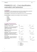
Plotting these graphically:
Using the equations above, each line is plotted on the graph.
The objective is to determine the coordinates of the points
where the lines intersect (the corner points). The grey shaded
area is the feasibility region.
The corner points can also be calculated mathematically by
pairing the lines and solving for X and Y, as follows:
Y ≤ -X + 3 Y ≤ -X + 3 Y ≤ 2X
Y ≤ 2X Y≥X-1 Y≥X-1
-X + 3 = 2X -X + 3 = X – 1 2X = X – 1
3X = 3 2X = 4 X = -1
X=1 X=2
Y = (2)(1) Y=2-1 Y = (2)(-1)
Y=2 Y=1 Y = -2
Corner point (1,2) Corner point (2,1) Corner point (-1,-2)
The maximum and minimum values of the optimization equation will be on the corners of the
feasibility region. Hence, we insert the coordinates above into the objective function to see
which coordinates yield the highest and lowest values:
Coordinates Z-Value
(1,2) Z = 3X + 3Y
= [2 X 1] + [3 X 2]
=2+6
=8
(2,1) Z = 2X + 3Y
= [2 X 2] + [3 X 1]
=4+3
=7
(-1,-2) Z = 2X + 3Y
= [2 X -1] + [3 X -2]
= -2 - 6
= -8
So, the max of Z = 8 occurs at (1,2) and the min of Z = -8 occurs at (-1,-2)
2
FINM6222 LU4 – Linear Programming
4.1 Intro
Linear Programming = mathematical method used to find the optimal solution in allocating
limited resources to achieve max profit or min costs
The following assumptions apply when using linear programming:
- the constraints (scarce resources) and objective functions are linear - i.e. the value of
the objective function and the responses of the constraints are proportional to the
level of activity
- the values of decision variables are divisible
- the coefficients are certain and representative of the population
- data, used in formulating the linear programme, is available.
4.2 Linear Programming Equations
The basic components in linear programming include:
- n variables (x1, x2)
- Linear inequalities / equalities within these variables (2x1 + 3x2 ≤ 4, 0 ≤ x1 ≤2 etc)
- Linear objective function (x1 + 2x2 = z)
Linear programming equations can be solved by plotting them graphically and determining
the coordinates of the corners of the feasibility region. These points are the tested in the
objective function (optimization equation)
Example 4.1
Find the min and max values of Z = 2X + 3Y (the objective function) subject to the following
constraints:
- 4X + 4Y ≤ 12
- 2X – Y ≥ 0
- X–Y≤1
The area within which the constraint lines intersect is called the ‘feasibility region’. The
formula Z = 2X + 3Y is the ‘optimization equation’ (or objective function). An objective
function is maximized on the last corner of the feasibility region before exiting that feasibility
region.
Our objective is to find the (X,Y) coordinates or corner points of the feasibility regions that
give rise to the lowest and highest values of Z.
The 1st step is to solve each inequality for their graphed equivalent forms as follows:
4X + 4Y ≤ 12 Y ≤ -X + 3
2X – Y ≥ 0 Y ≤ 2X
X – Y ≤ 1 Y ≥ X - 1
1
, FINM6222 LU4
Plotting these graphically:
Using the equations above, each line is plotted on the graph.
The objective is to determine the coordinates of the points
where the lines intersect (the corner points). The grey shaded
area is the feasibility region.
The corner points can also be calculated mathematically by
pairing the lines and solving for X and Y, as follows:
Y ≤ -X + 3 Y ≤ -X + 3 Y ≤ 2X
Y ≤ 2X Y≥X-1 Y≥X-1
-X + 3 = 2X -X + 3 = X – 1 2X = X – 1
3X = 3 2X = 4 X = -1
X=1 X=2
Y = (2)(1) Y=2-1 Y = (2)(-1)
Y=2 Y=1 Y = -2
Corner point (1,2) Corner point (2,1) Corner point (-1,-2)
The maximum and minimum values of the optimization equation will be on the corners of the
feasibility region. Hence, we insert the coordinates above into the objective function to see
which coordinates yield the highest and lowest values:
Coordinates Z-Value
(1,2) Z = 3X + 3Y
= [2 X 1] + [3 X 2]
=2+6
=8
(2,1) Z = 2X + 3Y
= [2 X 2] + [3 X 1]
=4+3
=7
(-1,-2) Z = 2X + 3Y
= [2 X -1] + [3 X -2]
= -2 - 6
= -8
So, the max of Z = 8 occurs at (1,2) and the min of Z = -8 occurs at (-1,-2)
2