

Empirical Methods in Finance Part 2
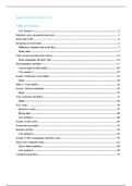
Table of Contents
Live session 1 ........................................................................................................................................... 3
Definition and conceptual framework......................................................................................................... 5
Extra video ATE ........................................................................................................................................... 6
Designing an event study ............................................................................................................................. 6
Difference calendar and event time....................................................................................................... 7
Stata codes ............................................................................................................................................... 7
Video normal and abnormal returns ......................................................................................................... 12
Stata commands AR and CAR ............................................................................................................ 14
Joint hypothesis problem ........................................................................................................................... 17
Canvas quizzes main points ................................................................................................................. 18
Live session 2 ......................................................................................................................................... 19
Lecture 3 Inference event studies .............................................................................................................. 23
Stata ....................................................................................................................................................... 25
Slides 2: event studies ................................................................................................................................ 26
Lecture 3 heteroscedasticity ....................................................................................................................... 28
Stata ....................................................................................................................................................... 31
Cross sectional correlation ........................................................................................................................ 32
Stata ....................................................................................................................................................... 35
Few events .................................................................................................................................................. 36
Stata few events..................................................................................................................................... 37
Recap quiz ............................................................................................................................................. 38
Live session 3 ......................................................................................................................................... 40
Lecture 4: time series ................................................................................................................................. 46
Trend and seasonality ................................................................................................................................ 47
Dynamic models ......................................................................................................................................... 50
Live session 4 ......................................................................................................................................... 55
Lecture 5: OLS assumptions and time series ............................................................................................ 59
Time series estimation Stata ...................................................................................................................... 64
Extra videos intuition ........................................................................................................................... 64
Live session 5 ......................................................................................................................................... 65
Assignment questions................................................................................................................................. 70
,Lecture 6: serial correlation and strong dependence ............................................................................... 71
Extra video random walk..................................................................................................................... 73
Serial correlation .................................................................................................................................. 73
Serial correlation testing ...................................................................................................................... 79
Stata Breusch-Godfrey ......................................................................................................................... 79
Class quiz summary.............................................................................................................................. 79
Live session 6 – serial correlation and persistent processes .............................................................. 84
Lecture 7 Time series models..................................................................................................................... 87
Time series processes ............................................................................................................................ 87
Selecting the right model ...................................................................................................................... 92
Stata ....................................................................................................................................................... 95
Live session 7.............................................................................................................................................. 96
Assignment for practice notes.................................................................................................................... 96
Lecture 8: Forecasting basics .................................................................................................................... 97
Model selection.................................................................................................................................... 100
Answers to the quiz: ........................................................................................................................... 101
Lecture 9 Stochastic volatility .................................................................................................................. 102
Stylized facts........................................................................................................................................ 102
Stochastic volatility with dice and coins ........................................................................................... 102
GARCH models .................................................................................................................................. 103
GARCH ............................................................................................................................................... 104
Leverage effects................................................................................................................................... 104
GARCH-in-mean model..................................................................................................................... 104
Live session block 8 and 9........................................................................................................................ 105
One step forecast................................................................................................................................. 105
Two step forecast → easy ................................................................................................................... 105
Two step forecast → long route ......................................................................................................... 106
................................ 106
Live session block 10 ................................................................................................................................ 106
Live session Mock exam .......................................................................................................................... 108
EXAM preparation................................................................................................................................... 109
Block 12: Live session .............................................................................................................................. 118
,Live session 1
𝐸(𝑎 + 𝑏𝑥 + 𝑐𝑦) = 𝑎 + 𝑏𝐸(𝑥) + 𝑐𝐸(𝑦)
𝑉𝑎𝑟(𝑎 + 𝑏𝑥 + 𝑐𝑦) = 0 + 𝑏 2 𝑉𝑎𝑟(𝑥) + 𝑐 2 𝑉𝑎𝑟(𝑦) + 2 ∗ 𝑏 ∗ 𝑐 ∗ 𝐶𝑜𝑣(𝑥, 𝑦)
𝐶𝑜𝑣(𝑎 + 𝑏𝑥 + 𝑐𝑦, 𝑥) = 𝐶𝑜𝑣(𝑎, 𝑥) + 𝑏 ∗ 𝐶𝑜𝑣(𝑥, 𝑥) + 𝑐 ∗ 𝐶𝑜𝑣(𝑦, 𝑥)
𝐶𝑜𝑣(𝑎, 𝑥) = 0, since a is a constant.
𝐶𝑜𝑣(𝑥, 𝑥) = 𝑉𝑎𝑟(𝑥)
𝐶𝑜𝑣(𝑦, 𝑥) = 𝐶𝑜𝑣(𝑥, 𝑦)
𝐶𝑜𝑣(𝑥, 𝑦)
𝐶𝑜𝑟𝑟(𝑥, 𝑦) =
√𝑉𝑎𝑟(𝑥) ∗ 𝑉𝑎𝑟(𝑦)
- Correlation is NOT a linear operator. This is why it falls between 0 and 1.
OLS
𝑦 = 𝛼 + 𝛽𝑥 + 𝜀
𝐶𝑜𝑣 (𝑥, 𝑦) 𝑉𝑎𝑟(𝑥)
𝛽̂ = = 𝐶𝑜𝑟𝑟(𝑥, 𝑦) ∗ √
𝑉𝑎𝑟(𝑥) 𝑉𝑎𝑟(𝑦)
- Variance of y and x is the same for event studies, so the second formula might be easier to use.
𝜀̂ = 𝐸(𝑦 − 𝛼̂ + ̂𝛽 𝑥) = 0
- Residual for OLS is ALWAYS 0.
𝛼̂ = 𝐸(𝑦) − 𝛽 ∗ 𝐸(𝑥)
Consistent: beta hat approaches beta when the sample size increases.
- Consistency is a property of the estimator but NOT of estimates.
Unbiased: the expected value of beta hat is equal to the true beta.
Efficiency: Var(beta_hat) < Var(beta_tilda)
̂
𝑉𝑎𝑟(𝛽)
IFFF ̃
𝑉𝑎𝑟(𝛾
→ 𝑐 < 1, as sample size increases.
1 1
𝑉1 = ∑(𝑥𝑖 − 𝑥)2 𝑎𝑛𝑑 𝑉2 = ∑(𝑥𝑖 − 𝑥)2
𝑁 𝑁−1
Differences two estimators of the variance:
- Both are consistent.
- V2 is unbiased but V1 has bias.
o Use V2 for small sample sizes.
- V1 is more efficient than V2.
o Use for large sample sizes.
V1 can never be BLUE, because it is biased.
- BLUE: Best Linear Unbiased Estimator.
, Conditioning: we take a subset of the sample and we take a moment in the subset of the sample.
You have 5 squares with different colors and each square has a color.
(8 + 1)
𝐸(𝑛𝑢𝑚𝑏𝑒𝑟|𝑐𝑜𝑙𝑜𝑟 = 𝑟𝑒𝑑) = = 4.5
2
10
𝐸(𝑛𝑢𝑚𝑏𝑒𝑟|𝑐𝑜𝑙𝑜𝑟 = 𝑔𝑟𝑒𝑒𝑛) = = 3.3
3
2 3
𝐸(𝑛𝑢𝑚𝑏𝑒𝑟) = 2.5 ∗ ( ) + 3.3 ∗ ( ) = 3.8
5 5
∑ 𝑛𝑢𝑚𝑏𝑒𝑟 𝑖𝑛 𝑠𝑞𝑢𝑎𝑟𝑒 2 ∑ 𝑛𝑢𝑚𝑏𝑒𝑟𝑠 𝑜𝑛 𝑠𝑞𝑢𝑎𝑟𝑒𝑠 2
𝑉(𝑛𝑢𝑚𝑏𝑒𝑟) = 𝑡𝑜𝑡𝑎𝑙 𝑛𝑢𝑚𝑏𝑒𝑟 𝑜𝑓 𝑠𝑞𝑢𝑎𝑟𝑒𝑠
− ( 𝑡𝑜𝑡𝑎𝑙 𝑛𝑢𝑚𝑏𝑒𝑟 𝑜𝑓 𝑠𝑞𝑢𝑎𝑟𝑒𝑠)
64+1 8+1 2
𝑉(𝑛𝑢𝑚𝑏𝑒𝑟|𝑐𝑜𝑙𝑜𝑟 = 𝑟𝑒𝑑) = 2
− ( 2
) = 12.25
25 + 4 + 9 5 + 2 + 3 2 14
𝑉(𝑛𝑢𝑚𝑏𝑒𝑟|𝑐𝑜𝑙𝑜𝑟 = 𝑔𝑟𝑒𝑒𝑛) = −( ) =
3 3 9
2 3 14 175
𝐸(𝑛𝑢𝑚𝑏𝑒𝑟|𝑐𝑜𝑙𝑜𝑟) = ∗ 12.25 + ∗ = ≈ 5.8
5 5 9 30
- We haven’t computed the risk before knowing the color. We have calculated the average risk
with knowing the color. So, there is still some risk there. As a result, it is an approximation.
We can, however, determine the true value by covering these steps:
2
𝑉(𝐸(𝑛𝑢𝑚𝑏𝑒𝑟|𝑐𝑜𝑙𝑜𝑟)) = 𝐸(𝐸(𝑛𝑢𝑚𝑏𝑒𝑟|𝑐𝑜𝑙𝑜𝑟)2 ) − 𝐸(𝐸(𝑛𝑢𝑚𝑏𝑒𝑟|𝑐𝑜𝑙𝑜𝑟))
2 10 2 3
𝑉(𝐸(𝑛𝑢𝑚𝑏𝑒𝑟|𝑐𝑜𝑙𝑜𝑟)) = 4.52 ∗ + ( ) ∗ − 3.82 = 0.326
5 3 5
Right result = 0.326 + 5.8 = 6.126
Law of total expectation:
𝐸(𝑦) = 𝐸(𝐸(𝑦|𝑥)) = ∑ 𝐸(𝑦|𝑥 = 𝑥𝑖 ) ∗ 𝑃(𝑥 = 𝑥𝑖 )
Law total variance:
𝑉(𝑦) = 𝑉(𝐸(𝑦|𝑥)) + 𝐸(𝑉(𝑦|𝑥))
- Expected idiosyncratic volatility
Table of Contents
Live session 1 ........................................................................................................................................... 3
Definition and conceptual framework......................................................................................................... 5
Extra video ATE ........................................................................................................................................... 6
Designing an event study ............................................................................................................................. 6
Difference calendar and event time....................................................................................................... 7
Stata codes ............................................................................................................................................... 7
Video normal and abnormal returns ......................................................................................................... 12
Stata commands AR and CAR ............................................................................................................ 14
Joint hypothesis problem ........................................................................................................................... 17
Canvas quizzes main points ................................................................................................................. 18
Live session 2 ......................................................................................................................................... 19
Lecture 3 Inference event studies .............................................................................................................. 23
Stata ....................................................................................................................................................... 25
Slides 2: event studies ................................................................................................................................ 26
Lecture 3 heteroscedasticity ....................................................................................................................... 28
Stata ....................................................................................................................................................... 31
Cross sectional correlation ........................................................................................................................ 32
Stata ....................................................................................................................................................... 35
Few events .................................................................................................................................................. 36
Stata few events..................................................................................................................................... 37
Recap quiz ............................................................................................................................................. 38
Live session 3 ......................................................................................................................................... 40
Lecture 4: time series ................................................................................................................................. 46
Trend and seasonality ................................................................................................................................ 47
Dynamic models ......................................................................................................................................... 50
Live session 4 ......................................................................................................................................... 55
Lecture 5: OLS assumptions and time series ............................................................................................ 59
Time series estimation Stata ...................................................................................................................... 64
Extra videos intuition ........................................................................................................................... 64
Live session 5 ......................................................................................................................................... 65
Assignment questions................................................................................................................................. 70
,Lecture 6: serial correlation and strong dependence ............................................................................... 71
Extra video random walk..................................................................................................................... 73
Serial correlation .................................................................................................................................. 73
Serial correlation testing ...................................................................................................................... 79
Stata Breusch-Godfrey ......................................................................................................................... 79
Class quiz summary.............................................................................................................................. 79
Live session 6 – serial correlation and persistent processes .............................................................. 84
Lecture 7 Time series models..................................................................................................................... 87
Time series processes ............................................................................................................................ 87
Selecting the right model ...................................................................................................................... 92
Stata ....................................................................................................................................................... 95
Live session 7.............................................................................................................................................. 96
Assignment for practice notes.................................................................................................................... 96
Lecture 8: Forecasting basics .................................................................................................................... 97
Model selection.................................................................................................................................... 100
Answers to the quiz: ........................................................................................................................... 101
Lecture 9 Stochastic volatility .................................................................................................................. 102
Stylized facts........................................................................................................................................ 102
Stochastic volatility with dice and coins ........................................................................................... 102
GARCH models .................................................................................................................................. 103
GARCH ............................................................................................................................................... 104
Leverage effects................................................................................................................................... 104
GARCH-in-mean model..................................................................................................................... 104
Live session block 8 and 9........................................................................................................................ 105
One step forecast................................................................................................................................. 105
Two step forecast → easy ................................................................................................................... 105
Two step forecast → long route ......................................................................................................... 106
................................ 106
Live session block 10 ................................................................................................................................ 106
Live session Mock exam .......................................................................................................................... 108
EXAM preparation................................................................................................................................... 109
Block 12: Live session .............................................................................................................................. 118
,Live session 1
𝐸(𝑎 + 𝑏𝑥 + 𝑐𝑦) = 𝑎 + 𝑏𝐸(𝑥) + 𝑐𝐸(𝑦)
𝑉𝑎𝑟(𝑎 + 𝑏𝑥 + 𝑐𝑦) = 0 + 𝑏 2 𝑉𝑎𝑟(𝑥) + 𝑐 2 𝑉𝑎𝑟(𝑦) + 2 ∗ 𝑏 ∗ 𝑐 ∗ 𝐶𝑜𝑣(𝑥, 𝑦)
𝐶𝑜𝑣(𝑎 + 𝑏𝑥 + 𝑐𝑦, 𝑥) = 𝐶𝑜𝑣(𝑎, 𝑥) + 𝑏 ∗ 𝐶𝑜𝑣(𝑥, 𝑥) + 𝑐 ∗ 𝐶𝑜𝑣(𝑦, 𝑥)
𝐶𝑜𝑣(𝑎, 𝑥) = 0, since a is a constant.
𝐶𝑜𝑣(𝑥, 𝑥) = 𝑉𝑎𝑟(𝑥)
𝐶𝑜𝑣(𝑦, 𝑥) = 𝐶𝑜𝑣(𝑥, 𝑦)
𝐶𝑜𝑣(𝑥, 𝑦)
𝐶𝑜𝑟𝑟(𝑥, 𝑦) =
√𝑉𝑎𝑟(𝑥) ∗ 𝑉𝑎𝑟(𝑦)
- Correlation is NOT a linear operator. This is why it falls between 0 and 1.
OLS
𝑦 = 𝛼 + 𝛽𝑥 + 𝜀
𝐶𝑜𝑣 (𝑥, 𝑦) 𝑉𝑎𝑟(𝑥)
𝛽̂ = = 𝐶𝑜𝑟𝑟(𝑥, 𝑦) ∗ √
𝑉𝑎𝑟(𝑥) 𝑉𝑎𝑟(𝑦)
- Variance of y and x is the same for event studies, so the second formula might be easier to use.
𝜀̂ = 𝐸(𝑦 − 𝛼̂ + ̂𝛽 𝑥) = 0
- Residual for OLS is ALWAYS 0.
𝛼̂ = 𝐸(𝑦) − 𝛽 ∗ 𝐸(𝑥)
Consistent: beta hat approaches beta when the sample size increases.
- Consistency is a property of the estimator but NOT of estimates.
Unbiased: the expected value of beta hat is equal to the true beta.
Efficiency: Var(beta_hat) < Var(beta_tilda)
̂
𝑉𝑎𝑟(𝛽)
IFFF ̃
𝑉𝑎𝑟(𝛾
→ 𝑐 < 1, as sample size increases.
1 1
𝑉1 = ∑(𝑥𝑖 − 𝑥)2 𝑎𝑛𝑑 𝑉2 = ∑(𝑥𝑖 − 𝑥)2
𝑁 𝑁−1
Differences two estimators of the variance:
- Both are consistent.
- V2 is unbiased but V1 has bias.
o Use V2 for small sample sizes.
- V1 is more efficient than V2.
o Use for large sample sizes.
V1 can never be BLUE, because it is biased.
- BLUE: Best Linear Unbiased Estimator.
, Conditioning: we take a subset of the sample and we take a moment in the subset of the sample.
You have 5 squares with different colors and each square has a color.
(8 + 1)
𝐸(𝑛𝑢𝑚𝑏𝑒𝑟|𝑐𝑜𝑙𝑜𝑟 = 𝑟𝑒𝑑) = = 4.5
2
10
𝐸(𝑛𝑢𝑚𝑏𝑒𝑟|𝑐𝑜𝑙𝑜𝑟 = 𝑔𝑟𝑒𝑒𝑛) = = 3.3
3
2 3
𝐸(𝑛𝑢𝑚𝑏𝑒𝑟) = 2.5 ∗ ( ) + 3.3 ∗ ( ) = 3.8
5 5
∑ 𝑛𝑢𝑚𝑏𝑒𝑟 𝑖𝑛 𝑠𝑞𝑢𝑎𝑟𝑒 2 ∑ 𝑛𝑢𝑚𝑏𝑒𝑟𝑠 𝑜𝑛 𝑠𝑞𝑢𝑎𝑟𝑒𝑠 2
𝑉(𝑛𝑢𝑚𝑏𝑒𝑟) = 𝑡𝑜𝑡𝑎𝑙 𝑛𝑢𝑚𝑏𝑒𝑟 𝑜𝑓 𝑠𝑞𝑢𝑎𝑟𝑒𝑠
− ( 𝑡𝑜𝑡𝑎𝑙 𝑛𝑢𝑚𝑏𝑒𝑟 𝑜𝑓 𝑠𝑞𝑢𝑎𝑟𝑒𝑠)
64+1 8+1 2
𝑉(𝑛𝑢𝑚𝑏𝑒𝑟|𝑐𝑜𝑙𝑜𝑟 = 𝑟𝑒𝑑) = 2
− ( 2
) = 12.25
25 + 4 + 9 5 + 2 + 3 2 14
𝑉(𝑛𝑢𝑚𝑏𝑒𝑟|𝑐𝑜𝑙𝑜𝑟 = 𝑔𝑟𝑒𝑒𝑛) = −( ) =
3 3 9
2 3 14 175
𝐸(𝑛𝑢𝑚𝑏𝑒𝑟|𝑐𝑜𝑙𝑜𝑟) = ∗ 12.25 + ∗ = ≈ 5.8
5 5 9 30
- We haven’t computed the risk before knowing the color. We have calculated the average risk
with knowing the color. So, there is still some risk there. As a result, it is an approximation.
We can, however, determine the true value by covering these steps:
2
𝑉(𝐸(𝑛𝑢𝑚𝑏𝑒𝑟|𝑐𝑜𝑙𝑜𝑟)) = 𝐸(𝐸(𝑛𝑢𝑚𝑏𝑒𝑟|𝑐𝑜𝑙𝑜𝑟)2 ) − 𝐸(𝐸(𝑛𝑢𝑚𝑏𝑒𝑟|𝑐𝑜𝑙𝑜𝑟))
2 10 2 3
𝑉(𝐸(𝑛𝑢𝑚𝑏𝑒𝑟|𝑐𝑜𝑙𝑜𝑟)) = 4.52 ∗ + ( ) ∗ − 3.82 = 0.326
5 3 5
Right result = 0.326 + 5.8 = 6.126
Law of total expectation:
𝐸(𝑦) = 𝐸(𝐸(𝑦|𝑥)) = ∑ 𝐸(𝑦|𝑥 = 𝑥𝑖 ) ∗ 𝑃(𝑥 = 𝑥𝑖 )
Law total variance:
𝑉(𝑦) = 𝑉(𝐸(𝑦|𝑥)) + 𝐸(𝑉(𝑦|𝑥))
- Expected idiosyncratic volatility


