

2022-04-24 13:51 Assignment4-Physics
Assignment 4: semiconductors and diodes
In [21]:
from IPython.display import YouTubeVideo
Problem 1
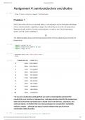
A NTC thermistor, like the one showed below, is a temperature sensor that takes advantage
of how a semiconductor negatively changes its conductivity as a function of temperature.
Suppose we take a piece of certain semiconductor. In order to use it as a temperature
sensor, we first need to calibrate it.
The following table shows experimental measurements of the conductivity as a function of
temperature.
In [2]:
import pandas as pd
import matplotlib.pyplot as plt
import numpy as np
In [3]:
data=pd.read_csv('data_assig.csv')
data
Out[3]: Temperature (K) σ (Ωm)^(-1)
0 620.0 4725.059345
1 560.0 2245.760723
2 510.0 1147.862882
3 480.0 800.000000
4 430.0 481.025258
5 410.0 395.444694
6 330.0 390.507083
7 290.0 382.718994
8 257.0 333.691619
9 232.0 258.023930
10 200.0 168.526251
* a) Use any visualization package that you want to meaningfully represent the
conductivity as a function of temperature, and approximately identify the temperature
intervals in which the semiconductor is found to be in the intrinsic, saturation, and
extrinsic regime. (In Python there are many packages for visualization: matplotlib,
seaborn, pandas... although you may use other software that you feel more
comfortable with).(5 points).
In [30]:
# conductivity as a function of temprature
file:///Users/bestricemossberg/Downloads/Assignment4-Physics.html 1/10
, 2022-04-24 13:51 Assignment4-Physics
# assign values to variables
x=data['Temperature (K)']
y=data["σ (Ωm)^(-1)"]
# fit model
theta = np.polyfit(x, y, 3)
# define values of y_line
y_line = theta[3] + theta[2]*pow(x, 1) + theta[1]*pow(x, 2) + theta[0]*pow(x,
# plot the graph
plt.scatter(x,y)
plt.plot(x, y_line, "orange")
plt.title("Conductivity as a function of temperature")
plt.xlabel("Temperature (K)")
plt.ylabel("σ (Ωm)^(-1)")
plt.show()
Method 1:
The conductivity of an intrinsic semiconductor increases as the temperature increases. For
an extrinsic semiconductor the conductivity decreases with the increase in temperature,
because the number of majority carriers is almost constant, while the mobility decreases,
which in turn leads to the conductivity decreasing.
Keeping this in mind, while looking at the plotted graph we can approximate the intrinsic
range from 620K to 410K, the saturation regime from 410K to 257K, and the extrinsic regime
from 257K to 200.
Method 2:
The image below shows the intrinsic, saturation, and extrinsic regime when log(σ) is plotted
as a function of 1/T. By plotting log(σ) as a function of 1/T we can compare the data to this
graph.
file:///Users/bestricemossberg/Downloads/Assignment4-Physics.html 2/10
Assignment 4: semiconductors and diodes
In [21]:
from IPython.display import YouTubeVideo
Problem 1
A NTC thermistor, like the one showed below, is a temperature sensor that takes advantage
of how a semiconductor negatively changes its conductivity as a function of temperature.
Suppose we take a piece of certain semiconductor. In order to use it as a temperature
sensor, we first need to calibrate it.
The following table shows experimental measurements of the conductivity as a function of
temperature.
In [2]:
import pandas as pd
import matplotlib.pyplot as plt
import numpy as np
In [3]:
data=pd.read_csv('data_assig.csv')
data
Out[3]: Temperature (K) σ (Ωm)^(-1)
0 620.0 4725.059345
1 560.0 2245.760723
2 510.0 1147.862882
3 480.0 800.000000
4 430.0 481.025258
5 410.0 395.444694
6 330.0 390.507083
7 290.0 382.718994
8 257.0 333.691619
9 232.0 258.023930
10 200.0 168.526251
* a) Use any visualization package that you want to meaningfully represent the
conductivity as a function of temperature, and approximately identify the temperature
intervals in which the semiconductor is found to be in the intrinsic, saturation, and
extrinsic regime. (In Python there are many packages for visualization: matplotlib,
seaborn, pandas... although you may use other software that you feel more
comfortable with).(5 points).
In [30]:
# conductivity as a function of temprature
file:///Users/bestricemossberg/Downloads/Assignment4-Physics.html 1/10
, 2022-04-24 13:51 Assignment4-Physics
# assign values to variables
x=data['Temperature (K)']
y=data["σ (Ωm)^(-1)"]
# fit model
theta = np.polyfit(x, y, 3)
# define values of y_line
y_line = theta[3] + theta[2]*pow(x, 1) + theta[1]*pow(x, 2) + theta[0]*pow(x,
# plot the graph
plt.scatter(x,y)
plt.plot(x, y_line, "orange")
plt.title("Conductivity as a function of temperature")
plt.xlabel("Temperature (K)")
plt.ylabel("σ (Ωm)^(-1)")
plt.show()
Method 1:
The conductivity of an intrinsic semiconductor increases as the temperature increases. For
an extrinsic semiconductor the conductivity decreases with the increase in temperature,
because the number of majority carriers is almost constant, while the mobility decreases,
which in turn leads to the conductivity decreasing.
Keeping this in mind, while looking at the plotted graph we can approximate the intrinsic
range from 620K to 410K, the saturation regime from 410K to 257K, and the extrinsic regime
from 257K to 200.
Method 2:
The image below shows the intrinsic, saturation, and extrinsic regime when log(σ) is plotted
as a function of 1/T. By plotting log(σ) as a function of 1/T we can compare the data to this
graph.
file:///Users/bestricemossberg/Downloads/Assignment4-Physics.html 2/10


