Georgia Tech ISYE6501 Week 2 HW, 100% pass rate
Georgia Tech ISYE6501 Week 2 HW, 100% pass rate, Document Content and Description Below ISYE6501 Week 2 HW Question 4.1 At my job we use clustering in an image system to understand the minerals that are coming into our processing facility. Comparing the images to known mineral images, the system can quantify the mineral content and monitor the colors of the minerals to compare to centroids of the clusters. Question 4.2 library(kernlab) library(ggplot2) ## Warning: package 'ggplot2' was built under R version 3.6.3 ## ## Attaching package: 'ggplot2' ## The following object is masked from 'package:kernlab': ## ## alpha library(kknn) ## Warning: package 'kknn' was built under R version 3.6.3 data<-("C:UsersColin ShumakerDesktopISYE6501Week 2data 4.2iri ", header = TRUE) data1 <-data[,1:4] head(data1) ## Sepal.Length Sepal.Width Petal.Length Petal.Width ## 1 5.1 3.5 1.4 0.2 ## 2 4.9 3.0 1.4 0.2 ## 3 4.7 3.2 1.3 0.2 ## 4 4.6 3.1 1.5 0.2 ## 5 5.0 3.6 1.4 0.2 ## 6 5.4 3.9 1.7 0.4species <-data[,5] kvalues <- rep(0,10) kx <- 1:10 (1000) for (r in 1:10){ ktest <- kmeans(data1,r,nstart=5, = 10) kx[r]<-r kvalues[r]<-ktest$ns } plot(kx,kvalues,type="b",xlab="Number of Clusters", ylab="Total Distance") (4) k <- kmeans(data1,3) cat("Predictors 1,2,3,4","n") ## Predictors 1,2,3,4 table(k$cluster,species)## species ## setosa versicolor virginica ## 1 0 48 14 ## 2 0 2 36 ## 3 50 0 0 (5) k1 <- kmeans(data1[,1:3],3) cat("Predictors 1,2,3","n") ## Predictors 1,2,3 table(k1$cluster,species) ## species ## setosa versicolor virginica ## 1 0 45 13 ## 2 50 0 0 ## 3 0 5 37 (6) k2 <- kmeans(data1[,2:4],3) cat("Predictors 2,3,4","n") ## Predictors 2,3,4 table(k2$cluster,species) ## species ## setosa versicolor virginica ## 1 0 48 5 ## 2 50 0 0 ## 3 0 2 45 (7) k3 <- kmeans(data1[,c(1,2,4)],3) cat("Predictors 1,2,4","n") ## Predictors 1,2,4table(k3$cluster,species) ## species ## setosa versicolor virginica ## 1 0 39 15 ## 2 0 11 35 ## 3 50 0 0 (8) k4 <- kmeans(data1[,c(1,3,4)],3) cat("Predictors 1,3,4","n") ## Predictors 1,3,4 table(k4$cluster,species) ## species ## setosa versicolor virginica ## 1 50 0 0 ## 2 0 2 36 ## 3 0 48 14 (9) k5 <- kmeans(data1[,3:4],3) cat("Predictors 3,4","n") ## Predictors 3,4 table(k5$cluster,species) ## species ## setosa versicolor virginica ## 1 0 2 46 ## 2 50 0 0 ## 3 0 48 4 ggplot(data,aes(x=Petal.Length,y=Petal.Width, col=Species))+ geom_point()# best k value is 3 based on the plot to find the best combination of predictors. The best accuracy is 96% showing that the best combination of predictors is 3 and 4. Evalu ating the clusters using h and shows the best response for spec ies Question 5.1 library(outliers) data1<-("C:UsersColin ShumakerDesktopISYE6501Week 2data 5.1usc ", header = TRUE) crimesort <- t(data1$Crime[order(data1$Crime)]) plot(seq(1:length(crimesort)),crimesort,xlab="Sort", ylab="Crime Rates")(crimesort, type=10) ## ## Grubbs test for one outlier ## ## data: crimeso
Written for
- Institution
- ISYE6501
- Module
- ISYE6501
Document information
- Uploaded on
- April 25, 2023
- Number of pages
- 10
- Written in
- 2022/2023
- Type
- Exam (elaborations)
- Contains
- Questions & answers
Subjects
-
georgia tech isye6501 week 2 hw
-
100 pass rate
-
document content and description below isye6501 week 2 hw question 41 at my job we use clustering in an image system to understand the minerals that a
Also available in package deal
