BIODIVERSITY
INTRODUCTION: DISCOVERY OF THE DIVERSITY
GRADIENT
Alexander von Humboldt: German geographer (1769-1859).
Humboldt Museum of Natural History (Berlin), Humboldt University (Berlin),
Humboldt Current and Humboldt Squid are all named after him.
A scientist and one of the last Renaissance Men (geologist, geographer,
meteorologist and natural historian). He decided he wanted to be an explorer –
planned to sail around the world, but this fell through. He wanted to explore
Egypt with Napoleon, and that fell through. Finally he ended up in Spain and set
off to explore South America for 5 years.
Travelled to Venezuela, discovered a new bird species, observed a meteor
shower, etc. and travelled to the newly-founded United States and discussed
science with President Thomas Jefferson. He spent 5 years away and 21 years
publishing his results. One of his greatest discoveries was mapping out the
climactic zones of the earth using isothermal lines. His systematic approach to
documenting the world revolutionised science and paved the way for Darwin and
Wallace and their discoveries.
His greatest observation was the Latitudinal Diversity Gradient: “the nearer we
approach the tropics, the greater the increase in the variety of structure, grace
of form, and mixture of colours…” Tropical rainforests have lots of species,
whereas Tundra does not – there are more species at low latitudes than high
latitudes.
DIVERSITY PATTERNS: Latitude, Altitude, Depth
and Area
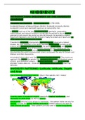
Map of diversity of mammal species: (blue = few species, red = many)
Diversity peaks in equatorial regions, especially tropical rainforests, and
decreases in cooler areas (as well as deserts).
Bird diversity (this isn’t just unique to mammals) – the pattern holds not only for
species, but also for genera, families and orders. Similar patterns are seen for
other animals and plants. These patterns are also seen in marine ecosystems.
, Other patterns: would we expect biodiversity to change with altitude? The
altitudinal gradient: in general, there are more species at low and mid-
altitudes, and fewer at high altitudes. This holds for both animals and plants.
There is also a depth gradient – as one descends into the ocean, there are
fewer species.
Area effects: how should the size of a land mass affect its diversity? Species-
Area Curves – larger islands have more species – there is a linear effect.
Why is this? We don’t have a definitive answer to these questions, but there are
theories.
MEASURING DIVERSITY: Alpha (local), Beta
(turnover), gamma (regional), evenness
Defining diversity – encompasses several concepts:
1. Total number of species for a given area: species richness, or alpha diversity
2. Relative abundance of species in that habitat, or evenness
3. Difference of a habitat from other habitats: turnover/ endemicity, or beta
diversity
4. Sum of everything in a region: regional diversity, or gamma diversity
1. Alpha diversity = the number of species found in a given habitat.
2. Relative abundance = some species may be very common, others may
be rare.
Often, a handful of common species dominate the assemblage. Most
species are rare.
Sampling – if many species are rare, how can we be sure we’ve found
them all? As you collect more individuals, you find more species. If we use
a computer to randomly draw subsamples from our data, we can see how
diversity goes up with larger sample size. The curve rises quickly as you
find the common species, then discovery slows since the easily found
species are rare, and you’re left with rare, harder to find species. When
the curve levels off, you’ve got everything.
Simpson’s Index: to calculate, you take the proportion of individuals a species
contributes, then square it, then do this for all species in your sample, and this
gives you Simpson’s index. A lower index means higher diversity, so often the
inverse is taken. There are lots of different kinds of metrics you can use.
3. Beta Diversity = endemism – how distinct is the fauna/flora from other
faunas or floras? Or as turnover – how quickly do species turn over from
one locality to another?
As we move from one place to another, some species drop out, and new
ones appear. Beta diversity is inversely proportional to shared species:
high beta means few shared species. Beta diversity tends to go up with
distance – as we move further away, beta diversity tends to increase.
Calculating Beta Diversity: as with evenness, there are indices to calculate
J = C / (C + U
beta diversity. Jaccard Similarity Index is one – for two habitats 1 and 21
this is:
Where C is the species common to both, U1 is species unique to habitat 1,
INTRODUCTION: DISCOVERY OF THE DIVERSITY
GRADIENT
Alexander von Humboldt: German geographer (1769-1859).
Humboldt Museum of Natural History (Berlin), Humboldt University (Berlin),
Humboldt Current and Humboldt Squid are all named after him.
A scientist and one of the last Renaissance Men (geologist, geographer,
meteorologist and natural historian). He decided he wanted to be an explorer –
planned to sail around the world, but this fell through. He wanted to explore
Egypt with Napoleon, and that fell through. Finally he ended up in Spain and set
off to explore South America for 5 years.
Travelled to Venezuela, discovered a new bird species, observed a meteor
shower, etc. and travelled to the newly-founded United States and discussed
science with President Thomas Jefferson. He spent 5 years away and 21 years
publishing his results. One of his greatest discoveries was mapping out the
climactic zones of the earth using isothermal lines. His systematic approach to
documenting the world revolutionised science and paved the way for Darwin and
Wallace and their discoveries.
His greatest observation was the Latitudinal Diversity Gradient: “the nearer we
approach the tropics, the greater the increase in the variety of structure, grace
of form, and mixture of colours…” Tropical rainforests have lots of species,
whereas Tundra does not – there are more species at low latitudes than high
latitudes.
DIVERSITY PATTERNS: Latitude, Altitude, Depth
and Area
Map of diversity of mammal species: (blue = few species, red = many)
Diversity peaks in equatorial regions, especially tropical rainforests, and
decreases in cooler areas (as well as deserts).
Bird diversity (this isn’t just unique to mammals) – the pattern holds not only for
species, but also for genera, families and orders. Similar patterns are seen for
other animals and plants. These patterns are also seen in marine ecosystems.
, Other patterns: would we expect biodiversity to change with altitude? The
altitudinal gradient: in general, there are more species at low and mid-
altitudes, and fewer at high altitudes. This holds for both animals and plants.
There is also a depth gradient – as one descends into the ocean, there are
fewer species.
Area effects: how should the size of a land mass affect its diversity? Species-
Area Curves – larger islands have more species – there is a linear effect.
Why is this? We don’t have a definitive answer to these questions, but there are
theories.
MEASURING DIVERSITY: Alpha (local), Beta
(turnover), gamma (regional), evenness
Defining diversity – encompasses several concepts:
1. Total number of species for a given area: species richness, or alpha diversity
2. Relative abundance of species in that habitat, or evenness
3. Difference of a habitat from other habitats: turnover/ endemicity, or beta
diversity
4. Sum of everything in a region: regional diversity, or gamma diversity
1. Alpha diversity = the number of species found in a given habitat.
2. Relative abundance = some species may be very common, others may
be rare.
Often, a handful of common species dominate the assemblage. Most
species are rare.
Sampling – if many species are rare, how can we be sure we’ve found
them all? As you collect more individuals, you find more species. If we use
a computer to randomly draw subsamples from our data, we can see how
diversity goes up with larger sample size. The curve rises quickly as you
find the common species, then discovery slows since the easily found
species are rare, and you’re left with rare, harder to find species. When
the curve levels off, you’ve got everything.
Simpson’s Index: to calculate, you take the proportion of individuals a species
contributes, then square it, then do this for all species in your sample, and this
gives you Simpson’s index. A lower index means higher diversity, so often the
inverse is taken. There are lots of different kinds of metrics you can use.
3. Beta Diversity = endemism – how distinct is the fauna/flora from other
faunas or floras? Or as turnover – how quickly do species turn over from
one locality to another?
As we move from one place to another, some species drop out, and new
ones appear. Beta diversity is inversely proportional to shared species:
high beta means few shared species. Beta diversity tends to go up with
distance – as we move further away, beta diversity tends to increase.
Calculating Beta Diversity: as with evenness, there are indices to calculate
J = C / (C + U
beta diversity. Jaccard Similarity Index is one – for two habitats 1 and 21
this is:
Where C is the species common to both, U1 is species unique to habitat 1,