
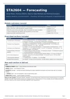
STA2604 — Forecasting
Study Notes, Formula Sheets, Step-by-Step Methods and Worked Examples
Based on: Bowerman, O’Connell & Koehler — Forecasting, Time Series, and Regression: An Applied Approach
Module outcomes covered
Outcome Where
Apply important concepts and methods in forecasting and detect forecasting errors Chapter 1 (1.1–1.5)
Build a regression model and perform residual analysis Chapters 3, 4, 5
Model the trend of time series data; detect and handle first-order correlation Chapter 6 (6.1–6.6)
Conduct multiplicative and additive decompositions of a time series Chapter 7 (7.1–7.3)
Apply exponential smoothing methods Chapter 8 (8.1, 8.3, 8.4)
Prescribed sections included
Chapter Sections
1.1 Forecasting and Data · 1.2 Forecasting Methods · 1.3 Errors in Forecasting · 1.4
1 Introduction to Forecasting
Choosing a Technique · 1.5 Overview of Quantitative Techniques
3.1 Model · 3.2 Least Squares Estimates · 3.3 Point Estimates/Predictions · 3.4
3 Simple Linear Regression Assumptions & Standard Error · 3.5 Testing Slope/Intercept · 3.6 Confidence &
Prediction Intervals · 3.7 r² and r · 3.8 F-test
4.1 Model · 4.2 Least Squares/Prediction · 4.3 Assumptions & Standard Error · 4.4 R²,
4 Multiple Linear Regression Adjusted R², F · 4.5 Testing a Variable · 4.6 CI/PI · 4.7 Quadratic · 4.8 Interaction · 4.9
Dummy Variables · 4.10 Partial F
5 Model Building & Residual 5.1 Model Building & Multicollinearity · 5.2 Residuals (simple) · 5.3 Residuals (multiple)
Analysis · 5.4 Outlying/Influential Observations
6.1 Polynomial Trend · 6.2 Autocorrelation (Durbin–Watson) · 6.3 Types of Seasonal
6 Time Series Regression Variation · 6.4 Dummy/Trig Seasonal Models · 6.5 Growth Curves · 6.6 First-Order
Autocorrelation
7 Decomposition Methods 7.1 Multiplicative · 7.2 Additive · 7.3 X-12-ARIMA
8 Exponential Smoothing 8.1 Simple · 8.3 Holt’s Trend Corrected · 8.4 Holt–Winters (additive and multiplicative)
How each section is laid out
KEY
FORMULA SHEET (blue) – every formula and rule you need.
STEPS (green) – the method in order.
EXAMPLE (orange) – worked example following the steps (textbook examples and extra ones with all numbers
shown).
⚠ TRICKY (red) – the non-standard / easy-to-get-wrong cases.
EXAM TIPS (purple) – end-of-chapter reminders.
Notes on the numbers. Examples labelled “Textbook” use the data/results printed in the book (checked against it). Examples
labelled “own data” were built for practice and computed exactly. Critical values (t, F) are rounded; use your tables/calculator in
the exam. Always use the notation and tables supplied in your assessments.
STA2604 Study Notes — based on Bowerman, O'Connell & Koehler, Forecasting, Time Series, and Regression Page 1
, Chapter 1 — An Introduction to Forecasting
Sections 1.1 – 1.5 | Outcome: apply forecasting concepts and detect forecasting errors
1.1 Forecasting and Data
FORMULA SHEET
Time series = chronological sequence of observations of one variable at (usually equally spaced) time points.
Cross-sectional data = values observed at one point in time (e.g. salary and GPA of last spring’s graduates).
Components of a time series: Trend (T) · Cycle (C) · Seasonal (S) · Irregular (I)
• Trend – long-run upward/downward movement. • Cycle – up-and-down swings around trend lasting 2–10+ years
(peak-to-peak), variable length.
• Seasonal – pattern that completes within one calendar year and repeats yearly (needs monthly/quarterly data).
• Irregular – erratic “left-over” movement after the other three are removed (strikes, storms, analyst error).
Forecasting strategy: (1) analyse past data → identify pattern, (2) extrapolate pattern. Only valid if the pattern
persists.
HOW TO IDENTIFY THE COMPONENTS
1. Look at the data: is it observed over time (time series) or at one time (cross-sectional)?
2. Plot it. Straight-line drift → trend; up/down waves longer than a year → cycle; repeating within-year shape →
seasonal.
3. Whatever is left unexplained is the irregular component.
4. Match the forecasting model to the components present (no single model fits all).
EXAMPLE — Classify each situation
(a) Monthly housing starts high in spring, low in winter → seasonal (weather, repeats each year).
(b) Sales rise steadily 8% a year for a decade → trend.
(c) Agricultural yield peaks about every 10 years (weather cycle) → cycle (longer than a year).
(d) A hurricane destroys a warehouse and one month’s sales collapse → irregular.
(e) Daily mean temperature over 3 years, Jan 1 to Dec 31 each year → seasonal + irregular.
⚠ TRICKY — A year of data cannot show seasonality
Question: a firm has one yearly total for each of 12 years. Can it estimate seasonal factors? No. Seasonal variation
needs monthly/quarterly (within-year) observations.
1.2 Forecasting Methods
FORMULA SHEET
Qualitative (judgemental) – expert opinion; used when data are scarce/non-existent (new product) or to predict
changes in pattern. Examples: subjective curve fitting (S-curve, product life cycle: growth → maturity → decline), the
Delphi method (panel of separated experts, repeated questionnaires, feedback of group opinion – consensus not
required), time-independent technological comparisons (primary trend in one area predicts another).
Quantitative – analyse historical data. Two kinds:
• Univariate model: forecasts using only past values of the series (assumes pattern continues; cannot show effect
of a policy change).
• Causal model: relates y (dependent) to other variables x1, x2,… (independent); needs forecasts of the x’s; lets
management test policies (price, advertising) but is harder to build.
UNIVARIATE OR CAUSAL?
1. Is there historical data? No → qualitative.
2. Does the formula for next period use only past values of the same series? → univariate.
3. Does it contain another variable (advertising, price, calls)? → causal.
EXAMPLE — Textbook Exercise 1.7 style
STA2604 Study Notes — based on Bowerman, O'Connell & Koehler, Forecasting, Time Series, and Regression Page 2
, (a) Sales(t+1) = 0.8·[Forecasted Sales(t)] + 0.2·[Sales(t)] → univariate (only sales history; this is simple
exponential smoothing with α = 0.2).
(b) Sales(t+1) = 500 + 2.5(Advertising in t) + 5(Customer calls in t) → causal (depends on other variables).
(c) Sales(t+1) = (1/t)·Σ Sales(i) → univariate (average of all past sales).
1.3 Errors in Forecasting
FORMULA SHEET
Forecast error et = yt − ŷt (actual − predicted).
MAD = Σ|et| / n MSE = Σ et² / n APEt = (|et| / yt)·100 MAPE = Σ APEt / n
Why not Σ et? positives and negatives cancel → near 0 even when errors are huge.
MSE punishes large errors much more (error 2 → 4, error 4 → 16). MAD treats all errors proportionally. MAPE is
unit-free so it compares series of different size (needs y > 0).
Error pattern check (plot et vs time): random scatter → model fits (only irregular left). Upward/downward trend
in errors → trend not captured. Repeating wave within a year → seasonal not captured. Longer wave → cycle not
captured.
Point forecast = single number. Prediction interval = range with stated confidence (e.g. 95%) that the actual
value lies in it.
Uses of MAD/MSE: (1) select the model whose “simulated” forecasts of past data have the smallest error; (2)
monitor a live system (tracking signals, Ch. 8).
HOW TO COMPUTE THE ACCURACY MEASURES
1. List actual yt and forecast ŷt side by side.
2. Compute et = yt − ŷt for every period.
3. MAD: take absolute values, add, divide by n. MSE: square, add, divide by n.
4. MAPE: divide each |et| by yt, ×100, then average.
5. Plot et over time and read the pattern (random = good).
⚠ TRICKY — Textbook Table 1.4 — two methods, MAD and MSE disagree
Actual y = 60, 64, 67. Method A predictions: 57, 61, 70. Method B predictions: 59, 65, 73.
A: e = [3, 3, -3]; |e| = 3,3,3 → MAD = 9/3 = 3.00; e² = 9,9,9 → MSE = 27/3 = 9.00.
B: e = [1, -1, -6]; |e| = 1,1,6 → MAD = 8/3 = 2.67; e² = 1,1,36 → MSE = 38/3 = 12.67.
Conclusion: A has the larger MAD (3 vs 2.67) but B has the larger MSE (12.67 vs 9) because B’s single big error
(−6) is squared. Choose B if you only care about average miss; choose A if large misses are costly.
EXAMPLE — Full calculation incl. MAPE (own numbers)
y = 25, 28, 30, 35 ; ŷ = 28, 29, 30, 33.
e = [-3, -1, 0, 2]; |e| = [np.int64(3), np.int64(1), np.int64(0), np.int64(2)]; e² = [np.int64(9), np.int64(1), np.int64(0),
np.int64(4)].
MAD = 6/4 = 1.50; MSE = 14/4 = 3.50.
APE = 12.00%, 3.57%, 0.00%, 5.71%; MAPE = 21.29/4 = 5.32%.
Note Σe = −3+(−1)+0+2 = −2 ≈ small although individual errors are up to 3 — the reason Σe is not used.
⚠ TRICKY — Reading error plots (Textbook Fig. 1.5)
(a) Errors scatter randomly about 0 → model fits the data pattern.
(b) Errors drift upward over time → the method does not account for trend.
(c) Errors repeat a within-year wave → seasonal pattern not accounted for.
(d) Errors show a long wave → cyclical pattern not accounted for.
Textbook Table 1.6 style: a model whose errors run +12,+15,+6,+5,… then −17,−21,−28,−34 then +5…+19 is
wave-like (cyclical pattern missed) and is inadequate even though some errors are small.
EXAMPLE — Interpreting a point vs prediction interval (Olympia Paper Towels)
Point forecast of week-121 sales: 258,889 rolls. 95% prediction interval: [238,517 ; 279,261].
STA2604 Study Notes — based on Bowerman, O'Connell & Koehler, Forecasting, Time Series, and Regression Page 3
Study Notes, Formula Sheets, Step-by-Step Methods and Worked Examples
Based on: Bowerman, O’Connell & Koehler — Forecasting, Time Series, and Regression: An Applied Approach
Module outcomes covered
Outcome Where
Apply important concepts and methods in forecasting and detect forecasting errors Chapter 1 (1.1–1.5)
Build a regression model and perform residual analysis Chapters 3, 4, 5
Model the trend of time series data; detect and handle first-order correlation Chapter 6 (6.1–6.6)
Conduct multiplicative and additive decompositions of a time series Chapter 7 (7.1–7.3)
Apply exponential smoothing methods Chapter 8 (8.1, 8.3, 8.4)
Prescribed sections included
Chapter Sections
1.1 Forecasting and Data · 1.2 Forecasting Methods · 1.3 Errors in Forecasting · 1.4
1 Introduction to Forecasting
Choosing a Technique · 1.5 Overview of Quantitative Techniques
3.1 Model · 3.2 Least Squares Estimates · 3.3 Point Estimates/Predictions · 3.4
3 Simple Linear Regression Assumptions & Standard Error · 3.5 Testing Slope/Intercept · 3.6 Confidence &
Prediction Intervals · 3.7 r² and r · 3.8 F-test
4.1 Model · 4.2 Least Squares/Prediction · 4.3 Assumptions & Standard Error · 4.4 R²,
4 Multiple Linear Regression Adjusted R², F · 4.5 Testing a Variable · 4.6 CI/PI · 4.7 Quadratic · 4.8 Interaction · 4.9
Dummy Variables · 4.10 Partial F
5 Model Building & Residual 5.1 Model Building & Multicollinearity · 5.2 Residuals (simple) · 5.3 Residuals (multiple)
Analysis · 5.4 Outlying/Influential Observations
6.1 Polynomial Trend · 6.2 Autocorrelation (Durbin–Watson) · 6.3 Types of Seasonal
6 Time Series Regression Variation · 6.4 Dummy/Trig Seasonal Models · 6.5 Growth Curves · 6.6 First-Order
Autocorrelation
7 Decomposition Methods 7.1 Multiplicative · 7.2 Additive · 7.3 X-12-ARIMA
8 Exponential Smoothing 8.1 Simple · 8.3 Holt’s Trend Corrected · 8.4 Holt–Winters (additive and multiplicative)
How each section is laid out
KEY
FORMULA SHEET (blue) – every formula and rule you need.
STEPS (green) – the method in order.
EXAMPLE (orange) – worked example following the steps (textbook examples and extra ones with all numbers
shown).
⚠ TRICKY (red) – the non-standard / easy-to-get-wrong cases.
EXAM TIPS (purple) – end-of-chapter reminders.
Notes on the numbers. Examples labelled “Textbook” use the data/results printed in the book (checked against it). Examples
labelled “own data” were built for practice and computed exactly. Critical values (t, F) are rounded; use your tables/calculator in
the exam. Always use the notation and tables supplied in your assessments.
STA2604 Study Notes — based on Bowerman, O'Connell & Koehler, Forecasting, Time Series, and Regression Page 1
, Chapter 1 — An Introduction to Forecasting
Sections 1.1 – 1.5 | Outcome: apply forecasting concepts and detect forecasting errors
1.1 Forecasting and Data
FORMULA SHEET
Time series = chronological sequence of observations of one variable at (usually equally spaced) time points.
Cross-sectional data = values observed at one point in time (e.g. salary and GPA of last spring’s graduates).
Components of a time series: Trend (T) · Cycle (C) · Seasonal (S) · Irregular (I)
• Trend – long-run upward/downward movement. • Cycle – up-and-down swings around trend lasting 2–10+ years
(peak-to-peak), variable length.
• Seasonal – pattern that completes within one calendar year and repeats yearly (needs monthly/quarterly data).
• Irregular – erratic “left-over” movement after the other three are removed (strikes, storms, analyst error).
Forecasting strategy: (1) analyse past data → identify pattern, (2) extrapolate pattern. Only valid if the pattern
persists.
HOW TO IDENTIFY THE COMPONENTS
1. Look at the data: is it observed over time (time series) or at one time (cross-sectional)?
2. Plot it. Straight-line drift → trend; up/down waves longer than a year → cycle; repeating within-year shape →
seasonal.
3. Whatever is left unexplained is the irregular component.
4. Match the forecasting model to the components present (no single model fits all).
EXAMPLE — Classify each situation
(a) Monthly housing starts high in spring, low in winter → seasonal (weather, repeats each year).
(b) Sales rise steadily 8% a year for a decade → trend.
(c) Agricultural yield peaks about every 10 years (weather cycle) → cycle (longer than a year).
(d) A hurricane destroys a warehouse and one month’s sales collapse → irregular.
(e) Daily mean temperature over 3 years, Jan 1 to Dec 31 each year → seasonal + irregular.
⚠ TRICKY — A year of data cannot show seasonality
Question: a firm has one yearly total for each of 12 years. Can it estimate seasonal factors? No. Seasonal variation
needs monthly/quarterly (within-year) observations.
1.2 Forecasting Methods
FORMULA SHEET
Qualitative (judgemental) – expert opinion; used when data are scarce/non-existent (new product) or to predict
changes in pattern. Examples: subjective curve fitting (S-curve, product life cycle: growth → maturity → decline), the
Delphi method (panel of separated experts, repeated questionnaires, feedback of group opinion – consensus not
required), time-independent technological comparisons (primary trend in one area predicts another).
Quantitative – analyse historical data. Two kinds:
• Univariate model: forecasts using only past values of the series (assumes pattern continues; cannot show effect
of a policy change).
• Causal model: relates y (dependent) to other variables x1, x2,… (independent); needs forecasts of the x’s; lets
management test policies (price, advertising) but is harder to build.
UNIVARIATE OR CAUSAL?
1. Is there historical data? No → qualitative.
2. Does the formula for next period use only past values of the same series? → univariate.
3. Does it contain another variable (advertising, price, calls)? → causal.
EXAMPLE — Textbook Exercise 1.7 style
STA2604 Study Notes — based on Bowerman, O'Connell & Koehler, Forecasting, Time Series, and Regression Page 2
, (a) Sales(t+1) = 0.8·[Forecasted Sales(t)] + 0.2·[Sales(t)] → univariate (only sales history; this is simple
exponential smoothing with α = 0.2).
(b) Sales(t+1) = 500 + 2.5(Advertising in t) + 5(Customer calls in t) → causal (depends on other variables).
(c) Sales(t+1) = (1/t)·Σ Sales(i) → univariate (average of all past sales).
1.3 Errors in Forecasting
FORMULA SHEET
Forecast error et = yt − ŷt (actual − predicted).
MAD = Σ|et| / n MSE = Σ et² / n APEt = (|et| / yt)·100 MAPE = Σ APEt / n
Why not Σ et? positives and negatives cancel → near 0 even when errors are huge.
MSE punishes large errors much more (error 2 → 4, error 4 → 16). MAD treats all errors proportionally. MAPE is
unit-free so it compares series of different size (needs y > 0).
Error pattern check (plot et vs time): random scatter → model fits (only irregular left). Upward/downward trend
in errors → trend not captured. Repeating wave within a year → seasonal not captured. Longer wave → cycle not
captured.
Point forecast = single number. Prediction interval = range with stated confidence (e.g. 95%) that the actual
value lies in it.
Uses of MAD/MSE: (1) select the model whose “simulated” forecasts of past data have the smallest error; (2)
monitor a live system (tracking signals, Ch. 8).
HOW TO COMPUTE THE ACCURACY MEASURES
1. List actual yt and forecast ŷt side by side.
2. Compute et = yt − ŷt for every period.
3. MAD: take absolute values, add, divide by n. MSE: square, add, divide by n.
4. MAPE: divide each |et| by yt, ×100, then average.
5. Plot et over time and read the pattern (random = good).
⚠ TRICKY — Textbook Table 1.4 — two methods, MAD and MSE disagree
Actual y = 60, 64, 67. Method A predictions: 57, 61, 70. Method B predictions: 59, 65, 73.
A: e = [3, 3, -3]; |e| = 3,3,3 → MAD = 9/3 = 3.00; e² = 9,9,9 → MSE = 27/3 = 9.00.
B: e = [1, -1, -6]; |e| = 1,1,6 → MAD = 8/3 = 2.67; e² = 1,1,36 → MSE = 38/3 = 12.67.
Conclusion: A has the larger MAD (3 vs 2.67) but B has the larger MSE (12.67 vs 9) because B’s single big error
(−6) is squared. Choose B if you only care about average miss; choose A if large misses are costly.
EXAMPLE — Full calculation incl. MAPE (own numbers)
y = 25, 28, 30, 35 ; ŷ = 28, 29, 30, 33.
e = [-3, -1, 0, 2]; |e| = [np.int64(3), np.int64(1), np.int64(0), np.int64(2)]; e² = [np.int64(9), np.int64(1), np.int64(0),
np.int64(4)].
MAD = 6/4 = 1.50; MSE = 14/4 = 3.50.
APE = 12.00%, 3.57%, 0.00%, 5.71%; MAPE = 21.29/4 = 5.32%.
Note Σe = −3+(−1)+0+2 = −2 ≈ small although individual errors are up to 3 — the reason Σe is not used.
⚠ TRICKY — Reading error plots (Textbook Fig. 1.5)
(a) Errors scatter randomly about 0 → model fits the data pattern.
(b) Errors drift upward over time → the method does not account for trend.
(c) Errors repeat a within-year wave → seasonal pattern not accounted for.
(d) Errors show a long wave → cyclical pattern not accounted for.
Textbook Table 1.6 style: a model whose errors run +12,+15,+6,+5,… then −17,−21,−28,−34 then +5…+19 is
wave-like (cyclical pattern missed) and is inadequate even though some errors are small.
EXAMPLE — Interpreting a point vs prediction interval (Olympia Paper Towels)
Point forecast of week-121 sales: 258,889 rolls. 95% prediction interval: [238,517 ; 279,261].
STA2604 Study Notes — based on Bowerman, O'Connell & Koehler, Forecasting, Time Series, and Regression Page 3


