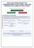
WGU C268 SPREADSHEETS OA
COMPREHENSIVE STUDY GUIDE | NEW 2026
VERSION WITH COMPLETE SOLUTIONS.
60 Questions with Answers and Detailed Rationales
100 PERCENT GUARANTEED PASS
INSTANT DOWNLOAD ANSWERS INCLUDED
IMPORTANCE OF THIS DOCUMENT
This comprehensive examination preparation guide has been meticulously developed to help you succeed in the
WGU C268 SPREADSHEETS OA COMPREHENSIVE STUDY GUIDE | NEW 2026 VERSION WITH
COMPLETE SOLUTIONS.. It contains 60 carefully selected questions that reflect the most current exam content
and testing strategies. Each question is accompanied by a correct answer and a detailed rationale that explains
the underlying pathophysiology, pharmacology, or clinical reasoning.
Self-Assessment – Test your knowledge and Exam Preparation – Familiarize yourself with the
identify areas requiring further question format and content
study areas
Concept Reinforcement – Deepen your Confidence Building – Develop test-taking
understanding through strategies and reduce
evidence-based exam anxiety
rationales
Time Management – Practice answering
questions under simulated
exam conditions
Review Summary 60 Questions
Foundations - Application - WGU C268 Spreadsheets OA Comprehensive Study Guide NEW 2026 Version
WITH Complete Solutions Spreadsheet Modeling AND DATA Analysis Microsoft Excel Undergraduate YEAR
3 / Advanced Spreadsheet Applications
All answers with rationales
,Table of Contents
Content Area Questions Key Topics
Spreadsheet Fundamentals 1-10 Formula, Sales, Correctly, Region, Product
Formulas AND Functions 11-20 Formula, YOU NEED, Sales, Correctly, Cells
DATA Visualization 21-30 YOU NEED, Formula, Sales, Model, Bonus
DATA Analysis 31-40 Sales, Function, Appropriate, YOU NEED, Dataset
What-if Analysis 41-50 Formula, Correctly, Sales, Monthly, Spreadsheet
Advanced Functions 51-60 Table, Model, Lookup, Ensure, Column
TOTAL 60 All questions include answers and detailed rationales
,Section A - Spreadsheet Fundamentals
Q1.
In a complex financial model, you need to return the sales figure for a given product and
region from a two-dimensional data table. Which formula correctly uses INDEX and
MATCH to retrieve the value where product names are in column A (A2:A100) and region
names are in row 1 (B1:Z1), with data in B2:Z100?
A. =INDEX(A1:Z100, MATCH(product, B. =INDEX(B2:Z100, MATCH(product,
A1:A100, 0), MATCH(region, A1:Z1, 0)) A2:A100, 0), MATCH(region, B1:Z1, 0))
C. =INDEX(B2:Z100, MATCH(product, D. =INDEX(A2:Z100, MATCH(product,
A2:A100, 1), MATCH(region, B1:Z1, 1)) A2:A100, 0), MATCH(region, B1:Z1, 0))
Correct: B - =INDEX(B2:Z100, MATCH(product, A2:A100, 0), MATCH(region, B1:Z1, 0))
Rationale:The correct formula uses INDEX on the data range (B2:Z100) only, and MATCH
with exact match (0) for both row and column lookups. Option B correctly references the data
range and the lookup arrays without including header row/column. Other options either
include headers in the INDEX range (A, D) or use approximate match (C), which is incorrect
for text labels.
Why the other answers are wrong:
A. Including headers in the INDEX range misaligns the row and column positions.
C. Using 1 (approximate match) is for numeric sorted data, not text product and region names.
D. Including the header row (A1:Z100) causes an offset, returning wrong values.
Reference: WGU C268 Spreadsheets Study Guide (2026), Module on Lookup & Reference Functions,
Ch. 2
Q2.
A company is evaluating a 5-year project with an initial investment of $50,000 and
expected annual net cash inflows of $15,000. Using Excel's NPV function with a discount
rate of 10%, which formula correctly computes the net present value, assuming cash flows
occur at the end of each year?
A. =NPV(10%, B2:B6) + B1 B. =NPV(10%, B1:B6)
C. =NPV(10%, B2:B6) - B1 D. =NPV(10%, B2:B6)
Correct: C - =NPV(10%, B2:B6) - B1
Rationale:Excel's NPV function assumes cash flows occur at the end of each period and
discounts the first cash flow by one period. The initial investment (B1) occurs at time 0 and
must be subtracted separately. Thus, =NPV(10%, B2:B6) - B1 is correct. Option A incorrectly
adds the initial investment, and B includes it in the NPV stream, misstating the timing.
Page 3
, Section A - Spreadsheet Fundamentals
Why the other answers are wrong:
A. Adding B1 treats the initial outflow as a positive inflow at time 0, which is incorrect.
B. Including the initial investment in the NPV function discounts it as if it occurs at year 1, not time 0.
D. Omitting the initial investment entirely ignores the initial cash outflow.
Reference: WGU C268 Spreadsheets Study Guide (2026), Financial Functions, Ch. 4
Q3.
Given a dataset with duplicate customer IDs, you need to create a formula that counts the
number of unique customers who made a purchase in the 'West' region. Which formula
correctly accomplishes this without using a helper column?
A. =SUMPRODUCT((region="West")/COUN B. =SUM(IF(region="West",
TIFS(customerID, customerID, region, 1/COUNTIF(customerID, customerID), 0))
"West"))
C. =COUNTIFS(region, "West", customerID, D. =SUMPRODUCT((region="West")*(COU
"<>"&"") NTIF(customerID, customerID)=1))
Correct: A - =SUMPRODUCT((region="West")/COUNTIFS(customerID, customerID, region,
"West"))
Rationale:The classic unique count formula with conditions uses SUMPRODUCT with
division by COUNTIFS that includes the same condition. This allocates fractional counts so
that each unique customer sums to 1. Option B works only if entered as an array formula
(CSE) and may fail without it. Option C counts all entries, not unique customers. Option D
counts only customers that appear exactly once, which is incorrect.
Why the other answers are wrong:
B. Requires Ctrl+Shift+Enter and does not correctly handle duplicate customers with the
condition.
C. Counts all customer IDs, not unique ones.
D. Only counts customers that occur exactly once, excluding those with multiple purchases.
Reference: WGU C268 Spreadsheets Study Guide (2026), Advanced Formulas, Ch. 3
Q4.
In a dashboard, you want to highlight cells in a sales table that are above the average for
their respective product category. Which Excel feature would you use to apply this
formatting dynamically without writing formulas in each cell?
A. Conditional Formatting with a formula rule B. Data Bars with a 'More Bar' rule.
referencing the category average.
C. Conditional Formatting with 'Top 10%' D. Format as Table with a custom style.
rule.
Correct: A - Conditional Formatting with a formula rule referencing the category average.
Page 4
COMPREHENSIVE STUDY GUIDE | NEW 2026
VERSION WITH COMPLETE SOLUTIONS.
60 Questions with Answers and Detailed Rationales
100 PERCENT GUARANTEED PASS
INSTANT DOWNLOAD ANSWERS INCLUDED
IMPORTANCE OF THIS DOCUMENT
This comprehensive examination preparation guide has been meticulously developed to help you succeed in the
WGU C268 SPREADSHEETS OA COMPREHENSIVE STUDY GUIDE | NEW 2026 VERSION WITH
COMPLETE SOLUTIONS.. It contains 60 carefully selected questions that reflect the most current exam content
and testing strategies. Each question is accompanied by a correct answer and a detailed rationale that explains
the underlying pathophysiology, pharmacology, or clinical reasoning.
Self-Assessment – Test your knowledge and Exam Preparation – Familiarize yourself with the
identify areas requiring further question format and content
study areas
Concept Reinforcement – Deepen your Confidence Building – Develop test-taking
understanding through strategies and reduce
evidence-based exam anxiety
rationales
Time Management – Practice answering
questions under simulated
exam conditions
Review Summary 60 Questions
Foundations - Application - WGU C268 Spreadsheets OA Comprehensive Study Guide NEW 2026 Version
WITH Complete Solutions Spreadsheet Modeling AND DATA Analysis Microsoft Excel Undergraduate YEAR
3 / Advanced Spreadsheet Applications
All answers with rationales
,Table of Contents
Content Area Questions Key Topics
Spreadsheet Fundamentals 1-10 Formula, Sales, Correctly, Region, Product
Formulas AND Functions 11-20 Formula, YOU NEED, Sales, Correctly, Cells
DATA Visualization 21-30 YOU NEED, Formula, Sales, Model, Bonus
DATA Analysis 31-40 Sales, Function, Appropriate, YOU NEED, Dataset
What-if Analysis 41-50 Formula, Correctly, Sales, Monthly, Spreadsheet
Advanced Functions 51-60 Table, Model, Lookup, Ensure, Column
TOTAL 60 All questions include answers and detailed rationales
,Section A - Spreadsheet Fundamentals
Q1.
In a complex financial model, you need to return the sales figure for a given product and
region from a two-dimensional data table. Which formula correctly uses INDEX and
MATCH to retrieve the value where product names are in column A (A2:A100) and region
names are in row 1 (B1:Z1), with data in B2:Z100?
A. =INDEX(A1:Z100, MATCH(product, B. =INDEX(B2:Z100, MATCH(product,
A1:A100, 0), MATCH(region, A1:Z1, 0)) A2:A100, 0), MATCH(region, B1:Z1, 0))
C. =INDEX(B2:Z100, MATCH(product, D. =INDEX(A2:Z100, MATCH(product,
A2:A100, 1), MATCH(region, B1:Z1, 1)) A2:A100, 0), MATCH(region, B1:Z1, 0))
Correct: B - =INDEX(B2:Z100, MATCH(product, A2:A100, 0), MATCH(region, B1:Z1, 0))
Rationale:The correct formula uses INDEX on the data range (B2:Z100) only, and MATCH
with exact match (0) for both row and column lookups. Option B correctly references the data
range and the lookup arrays without including header row/column. Other options either
include headers in the INDEX range (A, D) or use approximate match (C), which is incorrect
for text labels.
Why the other answers are wrong:
A. Including headers in the INDEX range misaligns the row and column positions.
C. Using 1 (approximate match) is for numeric sorted data, not text product and region names.
D. Including the header row (A1:Z100) causes an offset, returning wrong values.
Reference: WGU C268 Spreadsheets Study Guide (2026), Module on Lookup & Reference Functions,
Ch. 2
Q2.
A company is evaluating a 5-year project with an initial investment of $50,000 and
expected annual net cash inflows of $15,000. Using Excel's NPV function with a discount
rate of 10%, which formula correctly computes the net present value, assuming cash flows
occur at the end of each year?
A. =NPV(10%, B2:B6) + B1 B. =NPV(10%, B1:B6)
C. =NPV(10%, B2:B6) - B1 D. =NPV(10%, B2:B6)
Correct: C - =NPV(10%, B2:B6) - B1
Rationale:Excel's NPV function assumes cash flows occur at the end of each period and
discounts the first cash flow by one period. The initial investment (B1) occurs at time 0 and
must be subtracted separately. Thus, =NPV(10%, B2:B6) - B1 is correct. Option A incorrectly
adds the initial investment, and B includes it in the NPV stream, misstating the timing.
Page 3
, Section A - Spreadsheet Fundamentals
Why the other answers are wrong:
A. Adding B1 treats the initial outflow as a positive inflow at time 0, which is incorrect.
B. Including the initial investment in the NPV function discounts it as if it occurs at year 1, not time 0.
D. Omitting the initial investment entirely ignores the initial cash outflow.
Reference: WGU C268 Spreadsheets Study Guide (2026), Financial Functions, Ch. 4
Q3.
Given a dataset with duplicate customer IDs, you need to create a formula that counts the
number of unique customers who made a purchase in the 'West' region. Which formula
correctly accomplishes this without using a helper column?
A. =SUMPRODUCT((region="West")/COUN B. =SUM(IF(region="West",
TIFS(customerID, customerID, region, 1/COUNTIF(customerID, customerID), 0))
"West"))
C. =COUNTIFS(region, "West", customerID, D. =SUMPRODUCT((region="West")*(COU
"<>"&"") NTIF(customerID, customerID)=1))
Correct: A - =SUMPRODUCT((region="West")/COUNTIFS(customerID, customerID, region,
"West"))
Rationale:The classic unique count formula with conditions uses SUMPRODUCT with
division by COUNTIFS that includes the same condition. This allocates fractional counts so
that each unique customer sums to 1. Option B works only if entered as an array formula
(CSE) and may fail without it. Option C counts all entries, not unique customers. Option D
counts only customers that appear exactly once, which is incorrect.
Why the other answers are wrong:
B. Requires Ctrl+Shift+Enter and does not correctly handle duplicate customers with the
condition.
C. Counts all customer IDs, not unique ones.
D. Only counts customers that occur exactly once, excluding those with multiple purchases.
Reference: WGU C268 Spreadsheets Study Guide (2026), Advanced Formulas, Ch. 3
Q4.
In a dashboard, you want to highlight cells in a sales table that are above the average for
their respective product category. Which Excel feature would you use to apply this
formatting dynamically without writing formulas in each cell?
A. Conditional Formatting with a formula rule B. Data Bars with a 'More Bar' rule.
referencing the category average.
C. Conditional Formatting with 'Top 10%' D. Format as Table with a custom style.
rule.
Correct: A - Conditional Formatting with a formula rule referencing the category average.
Page 4