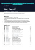
ASU -STP 311 Mock Exam 3 Applied Markets & Stochastic Processes 2026 Practice Mock Examination|actual
Questions with answers solution
ASU · STP 311
Quantitative Statistics · Practice Mock Examination
Mock Exam 03
Applied Markets & Stochastic Processes
Mechanism design, microstructure, stopping problems, and portfolio construction.
INSTRUCTIONS
• Time allowed: 3 hours. Questions: 21. Total: 100 points.
• Attempt every question. Show all algebraic steps; a correct final answer with no derivation earns partial
credit only.
• State any assumption you rely on, and note where an estimator is biased, inconsistent, or undefined.
• Worked solutions follow each question in this booklet. Cover them until you have committed to an answer.
• No calculator is required. Leave answers in closed form unless a number is explicitly requested.
QUESTION PAPER
Q01 [Estimation] Symmetric two-point mixture 5 pts
Q02 [Estimation] Endogenous regressor 5 pts
Q03 [Estimation] Correlation from two noisy proxies 5 pts
Q04 [Diagnostics] “ p = 0.01 means 99% chance the factor is real” 5 pts
Q05 [Diagnostics] OLS t-stats under heteroskedasticity 5 pts
Q06 [Diagnostics] Base-rate fallacy in a crash alarm 5 pts
Q07 [Applied] Censored return labels under a price limit 5 pts
Q08 [Applied] Variance-minimizing hedge ratio 5 pts
Q09 [Applied] Fill probability of a resting limit order 5 pts
Q10 [Applied] Reflection principle and the running maximum 5 pts
Q11 [Applied] Minimum-variance portfolio 5 pts
Q12 [Numerical] Variance of a linear combination (numerical) 5 pts
Q13 [Numerical] Delta method (numerical) 5 pts
Q14 [Distribution Theory] Geometric distribution moments 5 pts
Q15 [Market Making] Roll until a six: a market on the total 5 pts
Q16 [Market Making] Queue position and what a fill tells you 5 pts
Q17 [Group Markets] Doubles, and the room’s highest roll 4 pts
Q18 [Group Markets] Mean versus median of the room 4 pts
Q19 [Linear Algebra] Eigenvectors of a two-asset covariance 4 pts
Q20 [Linear Algebra] Cholesky: simulating correlated returns 4 pts
Q21 [Research Design] Perpetual futures funding and the basis 4 pts
,A5. Symmetric two-point mixture
Setup.
1
2
observation is normal with mean Sµ and variance 1. You observe only the values, never the
signs.
Derive an estimator of µ.
Solution.
The mean carries no signal. By the law of total expectation, conditioning on the sign,
E[Y] = E E[Y | S] = E[Sµ] = µ E[S] = µ (+1) 21 + (−1) 12 = 0.
So E[Y] = 0 for every µ; a method-of-moments estimator built on the first moment is useless.
Use the second moment. The sign entered linearly above; square it away. Conditional on S, the
observation has variance 1 and mean Sµ, so
2
E[Y2 | S] = Var(Y | S) + E[Y | S] = 1 + (Sµ)2 = 1 + S2µ2 = 1 + µ2,
using S2 = 1, which is free of S. Taking the expectation over S leaves it unchanged:
E[Y2] = 1 + µ2.
Estimator. Solve for µ2 and match the sample second moment:
r
µ2 = E[Y2] − 1 =⇒ | µ̂ | = max n1 ∑i Yi2 − 1, 0 .
Consistent by the law of large numbers; the sign of µ is unidentifiable because the mixture is sym-
metric about 0.
If the variance were unknown. One equation cannot fix two unknowns (µ, σ2), so add the fourth
moment. Conditional on S, a N (Sµ, σ2) variable has E[Y4 | S] = (Sµ)4 + 6(Sµ)2σ2 + 3σ4 = µ4 +
6µ2σ2 + 3σ4 (again free of S). So
E[Y2] = µ2 + σ2, E[Y4] = µ4 + 6µ2σ2 + 3σ4,
two equations solved jointly for (µ2, σ2) from the sample second and fourth moments. (Simulation
µ = 1.7: | µ̂ | = 1.70.)
10
, A13. Endogenous regressor
Setup.
The structural model is Y = βX + ε but Cov(X, ε) = 0 (both react to an unobserved shock). You
Show OLS is inconsistent and derive a consistent estimator of β.
Solution.
ˆ
ˆCov(X, Y)/Var(X),
OLS is inconsistent. The OLS setup gives slope b = ˆ converging to Cov(X, Y)/ Var(X).
Expand the numerator with the structural equation and bilinearity:
Cov(X, Y) = Cov(X, βX + ε) = β Cov(X, X) + Cov(X, ε) = β Var(X) + Cov(X, ε).
Dividing by Var(X),
p Cov(X, ε)
bˆ −
→ β+ ̸= β,
Var(X)
so the endogeneity term persists no matter how large the sample: OLS is inconsistent.
Use the instrument. The instrument’s two defining properties are relevance Cov(W, X) = 0 and
exclusion Cov(W, ε) = 0. Take the covariance of the structural equation with W:
Cov(W, Y) = Cov(W, βX + ε) = β Cov(W, X) + Cov(W, ε) = β Cov(W, X),
the last term vanishing by exclusion. Solve for β and replace population covariances by sample
versions:
C ô v (W , Y)
β̂IV = .
C ôv(W , X)
By the law of large numbers the sample covariances converge to their population values, so β̂ I V → β:
consistent.
Equivalent two-stage form. Regress X on W to obtain fitted values X̂ (the part of X driven by the ex-
ogenous W), then regress Y on X̂ ; the resulting slope equals β̂ I V above, because Cov(X̂ , Y)/ Var( X̂ ) re-
duces to Cov(W, Y)/ Cov(W, X) for a single instrument. Degenerate: if relevance is weak (Cov(W, X) ≈
0) the denominator is tiny and the estimator’s variance explodes — the weak-instrument problem.
19
Questions with answers solution
ASU · STP 311
Quantitative Statistics · Practice Mock Examination
Mock Exam 03
Applied Markets & Stochastic Processes
Mechanism design, microstructure, stopping problems, and portfolio construction.
INSTRUCTIONS
• Time allowed: 3 hours. Questions: 21. Total: 100 points.
• Attempt every question. Show all algebraic steps; a correct final answer with no derivation earns partial
credit only.
• State any assumption you rely on, and note where an estimator is biased, inconsistent, or undefined.
• Worked solutions follow each question in this booklet. Cover them until you have committed to an answer.
• No calculator is required. Leave answers in closed form unless a number is explicitly requested.
QUESTION PAPER
Q01 [Estimation] Symmetric two-point mixture 5 pts
Q02 [Estimation] Endogenous regressor 5 pts
Q03 [Estimation] Correlation from two noisy proxies 5 pts
Q04 [Diagnostics] “ p = 0.01 means 99% chance the factor is real” 5 pts
Q05 [Diagnostics] OLS t-stats under heteroskedasticity 5 pts
Q06 [Diagnostics] Base-rate fallacy in a crash alarm 5 pts
Q07 [Applied] Censored return labels under a price limit 5 pts
Q08 [Applied] Variance-minimizing hedge ratio 5 pts
Q09 [Applied] Fill probability of a resting limit order 5 pts
Q10 [Applied] Reflection principle and the running maximum 5 pts
Q11 [Applied] Minimum-variance portfolio 5 pts
Q12 [Numerical] Variance of a linear combination (numerical) 5 pts
Q13 [Numerical] Delta method (numerical) 5 pts
Q14 [Distribution Theory] Geometric distribution moments 5 pts
Q15 [Market Making] Roll until a six: a market on the total 5 pts
Q16 [Market Making] Queue position and what a fill tells you 5 pts
Q17 [Group Markets] Doubles, and the room’s highest roll 4 pts
Q18 [Group Markets] Mean versus median of the room 4 pts
Q19 [Linear Algebra] Eigenvectors of a two-asset covariance 4 pts
Q20 [Linear Algebra] Cholesky: simulating correlated returns 4 pts
Q21 [Research Design] Perpetual futures funding and the basis 4 pts
,A5. Symmetric two-point mixture
Setup.
1
2
observation is normal with mean Sµ and variance 1. You observe only the values, never the
signs.
Derive an estimator of µ.
Solution.
The mean carries no signal. By the law of total expectation, conditioning on the sign,
E[Y] = E E[Y | S] = E[Sµ] = µ E[S] = µ (+1) 21 + (−1) 12 = 0.
So E[Y] = 0 for every µ; a method-of-moments estimator built on the first moment is useless.
Use the second moment. The sign entered linearly above; square it away. Conditional on S, the
observation has variance 1 and mean Sµ, so
2
E[Y2 | S] = Var(Y | S) + E[Y | S] = 1 + (Sµ)2 = 1 + S2µ2 = 1 + µ2,
using S2 = 1, which is free of S. Taking the expectation over S leaves it unchanged:
E[Y2] = 1 + µ2.
Estimator. Solve for µ2 and match the sample second moment:
r
µ2 = E[Y2] − 1 =⇒ | µ̂ | = max n1 ∑i Yi2 − 1, 0 .
Consistent by the law of large numbers; the sign of µ is unidentifiable because the mixture is sym-
metric about 0.
If the variance were unknown. One equation cannot fix two unknowns (µ, σ2), so add the fourth
moment. Conditional on S, a N (Sµ, σ2) variable has E[Y4 | S] = (Sµ)4 + 6(Sµ)2σ2 + 3σ4 = µ4 +
6µ2σ2 + 3σ4 (again free of S). So
E[Y2] = µ2 + σ2, E[Y4] = µ4 + 6µ2σ2 + 3σ4,
two equations solved jointly for (µ2, σ2) from the sample second and fourth moments. (Simulation
µ = 1.7: | µ̂ | = 1.70.)
10
, A13. Endogenous regressor
Setup.
The structural model is Y = βX + ε but Cov(X, ε) = 0 (both react to an unobserved shock). You
Show OLS is inconsistent and derive a consistent estimator of β.
Solution.
ˆ
ˆCov(X, Y)/Var(X),
OLS is inconsistent. The OLS setup gives slope b = ˆ converging to Cov(X, Y)/ Var(X).
Expand the numerator with the structural equation and bilinearity:
Cov(X, Y) = Cov(X, βX + ε) = β Cov(X, X) + Cov(X, ε) = β Var(X) + Cov(X, ε).
Dividing by Var(X),
p Cov(X, ε)
bˆ −
→ β+ ̸= β,
Var(X)
so the endogeneity term persists no matter how large the sample: OLS is inconsistent.
Use the instrument. The instrument’s two defining properties are relevance Cov(W, X) = 0 and
exclusion Cov(W, ε) = 0. Take the covariance of the structural equation with W:
Cov(W, Y) = Cov(W, βX + ε) = β Cov(W, X) + Cov(W, ε) = β Cov(W, X),
the last term vanishing by exclusion. Solve for β and replace population covariances by sample
versions:
C ô v (W , Y)
β̂IV = .
C ôv(W , X)
By the law of large numbers the sample covariances converge to their population values, so β̂ I V → β:
consistent.
Equivalent two-stage form. Regress X on W to obtain fitted values X̂ (the part of X driven by the ex-
ogenous W), then regress Y on X̂ ; the resulting slope equals β̂ I V above, because Cov(X̂ , Y)/ Var( X̂ ) re-
duces to Cov(W, Y)/ Cov(W, X) for a single instrument. Degenerate: if relevance is weak (Cov(W, X) ≈
0) the denominator is tiny and the estimator’s variance explodes — the weak-instrument problem.
19