

Part 1 - Black Scholes Merton model
25 November 2025 14:17
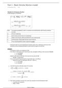
Valuation of a European call option
Underlying pays no dividends
N[d1] Cumulative probability Z will in a standard normal distribution (left-hand cumulative
normal)
S0 Price of underlying
σ SD of annual rate of return on underlying
E Option exercise price (discounted back to now continuously)
ρ Continuously compounded risk-free rate of interest
t Time remaining before option expiration in years
- Scaling for both d1 and d2 (dividing by σ√t) deals with some underlying continuous time
processes whose standard deviation evolves with the square root of time
EXAMPLE
- A company’s shares are trading at £2.98
- The return on the shares over several years has averaged 0.1945 pa, with variance 0.038280
σ = √0.038280
σ = 0.195653
- Options with expiry in 86 days’ time have exercise price £3.00
○ 86/365 = 0.2356 years
- The current bank 90-day annually compounded rate is 15.58% pa
○ Need to convert to continuous rate so ρ = ln(1+rd)
ρ = ln(1.1558)
ρ = 0.144793
Use the formula to calculate values for d1 and d2
Then find cumulative normals of d1 and d2 by using the normal distribution table
○ d1 and d2 are Z statistics
○ N[d1] = 0.633
Fiance v2 Page 1
, ○ N[d2] = 0.595
Then use the formula to give the value of the call option equal to £0.16
If we needed to use the BSM model to find put option price
- Recall the put-call parity:
S0 + P = Ee-rt + C
- So P = £0.08
Going back to Binomial briefly
- Consider an asset with current price S0, expected annual return μ and volatility σ
- One-period binomial model over small time-step ∆t with estimated real probability of an
upward movement in asset price, p*
NOT NEEDED AS A PROOF, JUST BACKGROUND
- Start with the expected price at the end of this period:
μ∆t
S0eμ∆t = p*S0u + (1 - p*)S0d p* = ⎯⎯⎯⎯⎯⎯
○ u and d represent up and down multiplier in up and down states
○ We have applied probabilities to the possible prices in the up and down states
- Then look at the variance of returns at the end of this period using Var[X] = E[X2] - (E[X])2 :
σ2∆t = p*u2 + (1 - p*)d2 - (p*u + (1 - p*)d)2
○ Substitute the above equation for p*
σ2∆t = eμ∆t (u + d) - ud - e2μ∆t
Cox, Ross and Rubenstein (1979) said that if we want to transit between binomial and continuous to
BSM, we can set up u and d in our equations to match volatility
- Can expand exponential functions as Maclaurin series and ignore the O[∆t 2+] terms:
○ Which gives:
u = eσ√∆t and d = ⎯
Convergence of binomial to BSM
EXAMPLE
S 120¢
σ 0.4
E 100¢
t 3 yrs
rf 5.00% pa
ρ 4.88% pa
- Rf would be used in the discrete binomial model, ρ would be used in the continuous time BSM
model
Given the above data, we can use CRR to deduce u and d for increasing number of periods in the
binomial model
- Depending on the time steps we use in the binomial model
Fiance v2 Page 2
25 November 2025 14:17
Valuation of a European call option
Underlying pays no dividends
N[d1] Cumulative probability Z will in a standard normal distribution (left-hand cumulative
normal)
S0 Price of underlying
σ SD of annual rate of return on underlying
E Option exercise price (discounted back to now continuously)
ρ Continuously compounded risk-free rate of interest
t Time remaining before option expiration in years
- Scaling for both d1 and d2 (dividing by σ√t) deals with some underlying continuous time
processes whose standard deviation evolves with the square root of time
EXAMPLE
- A company’s shares are trading at £2.98
- The return on the shares over several years has averaged 0.1945 pa, with variance 0.038280
σ = √0.038280
σ = 0.195653
- Options with expiry in 86 days’ time have exercise price £3.00
○ 86/365 = 0.2356 years
- The current bank 90-day annually compounded rate is 15.58% pa
○ Need to convert to continuous rate so ρ = ln(1+rd)
ρ = ln(1.1558)
ρ = 0.144793
Use the formula to calculate values for d1 and d2
Then find cumulative normals of d1 and d2 by using the normal distribution table
○ d1 and d2 are Z statistics
○ N[d1] = 0.633
Fiance v2 Page 1
, ○ N[d2] = 0.595
Then use the formula to give the value of the call option equal to £0.16
If we needed to use the BSM model to find put option price
- Recall the put-call parity:
S0 + P = Ee-rt + C
- So P = £0.08
Going back to Binomial briefly
- Consider an asset with current price S0, expected annual return μ and volatility σ
- One-period binomial model over small time-step ∆t with estimated real probability of an
upward movement in asset price, p*
NOT NEEDED AS A PROOF, JUST BACKGROUND
- Start with the expected price at the end of this period:
μ∆t
S0eμ∆t = p*S0u + (1 - p*)S0d p* = ⎯⎯⎯⎯⎯⎯
○ u and d represent up and down multiplier in up and down states
○ We have applied probabilities to the possible prices in the up and down states
- Then look at the variance of returns at the end of this period using Var[X] = E[X2] - (E[X])2 :
σ2∆t = p*u2 + (1 - p*)d2 - (p*u + (1 - p*)d)2
○ Substitute the above equation for p*
σ2∆t = eμ∆t (u + d) - ud - e2μ∆t
Cox, Ross and Rubenstein (1979) said that if we want to transit between binomial and continuous to
BSM, we can set up u and d in our equations to match volatility
- Can expand exponential functions as Maclaurin series and ignore the O[∆t 2+] terms:
○ Which gives:
u = eσ√∆t and d = ⎯
Convergence of binomial to BSM
EXAMPLE
S 120¢
σ 0.4
E 100¢
t 3 yrs
rf 5.00% pa
ρ 4.88% pa
- Rf would be used in the discrete binomial model, ρ would be used in the continuous time BSM
model
Given the above data, we can use CRR to deduce u and d for increasing number of periods in the
binomial model
- Depending on the time steps we use in the binomial model
Fiance v2 Page 2


