MTA II Notes
Lecture notes and Tutorials
This summary is based on the lecture slides for Measurement Theory and Assessment by Pelt (2025–
2026).
Week 1
Lecture 1 - Introduction to Psychometrics
Psychological Measurement
Measurement in psychology = the assignment of numerals to psychological characteristics of individuals
according to rules.
↳ Example: “I like to go to parties” → No = 0, Yes = 1.
The characteristic refers to an underlying psychological variable or construct (e.g., extraversion,
anxiety). The rules come from a defined test procedure (e.g., self-report items, behavioural tasks,
reaction times).
Psychometrics = the science of evaluating psychological tests → concerned with test properties such
as reliability, validity, and bias.
↳ It applies to all types of psychological measurement – not only self-report but also performance-
based or behavioural measures.
Psychologists need to know whether their measurement tools are:
• Reliable → consistent across time, items, or raters.
• Valid → actually measuring what they claim to measure.
• Fair (unbiased) → not disadvantaging certain groups.
Key questions include:
➢ “Is my test valid for this purpose?”
➢ “Is it reliable enough to draw conclusions?”
➢ “Are scores comparable across groups or situations?”
Latent and Observed Variables
Many psychological constructs are latent variables – they cannot be observed directly (e.g.,
depression, intelligence). We infer them through observable indicators such as responses,
performance, or physiological measures.
• Observable variables = responses to items or tasks (e.g., “I feel sad,” number of remembered
words).
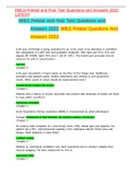
• Latent variable models use path diagrams:
o Latent variable → shown as a circle (unobservable).
o Observed items → shown as boxes.
o Arrows (→) represent the assumed causal direction from latent → observed.
Measurement error → every observed variable relates to the latent variable imperfectly.
↳ Hence, we always model an error term (in a small circle).
Page 1
,Roles of Theory, Statistics, and Causality
Theory: Psychological theory defines what should be measured and how it manifests.
o Example: ADHD theory → inattention + hyperactivity + impulsivity.
o Personality theory → Big Five (OCEAN) dimensions.
Theory guides:
1. Which latent constructs to include.
2. How to operationalize them into observable items.
3. Expectations about how items interrelate (dimensionality).
Statistics provides tools to examine individual differences in item responses. Core quantities: mean,
variance, covariance, correlation, and regression.
• Variance = spread of scores around the mean.
• Correlation = degree of standardized covariance between two variables. “How strongly are X
and Y related?”
• Covariance = indicates how much two variables change together. A positive covariance means
the variables tend to move in the same direction, while a negative covariance indicates they
move in opposite directions.
• Regression = estimation of relationships between a dependent variable and one or more
independent variables. “Can I predict Y if I know X?”
Regression models link latent and observed variables:
• Latent variable → item + error (b = strength of relationship).
Correlation does not imply causation → statistical association alone is not enough to interpret
meaning.
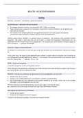
Skewness
Skewness tells you about the symmetry (or asymmetry) of a distribution — in other words, whether
the data are pulled to one side.
1. Positive Skew (Right-Skewed)
a. Tail on the right side
b. The right tail (higher values) is longer or fatter.
c. Most scores are low, with a few very high values pulling the mean upward.
d. Mean > Median > Mode
Example: Income, reaction times — a few people earn a lot, but most earn less.
Tip to remember:
The tail points to the direction of the skew — right tail → positive skew.
Page 2
, 2. Negative Skew (Left-Skewed)
a. Tail on the left side
b. The left tail (lower values) is longer or fatter.
c. Most scores are high, with a few low outliers pulling the mean downward.
d. Mean < Median < Mode
Example: Age at retirement — most retire around the same age, but a few retire very
early.
Symmetrical Distribution:
- No skew — looks like a bell curve (normal distribution).
- Mean = Median = Mode
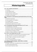
Kurtosis
Kurtosis describes the "tailedness" or peakedness" of a distribution = how heavy or light the tails are
compared to a normal distribution. A normal distribution is bell-shaped, has medium tails (neither too
thick nor thin). There are two types of kurtosis:
1. Positive kurtosis
a. Very tall peak and fat tails
b. Data are clustered tightly around the mean, but with more extreme outliers
c. Indicates more risks/variability in extremes
Example: Exam scores where most people get average marks, but a few get very high or
very low.
2. Negative kurtosis
a. Flat peak and thin tails
b. Values are spread out more evenly with fewer outliers
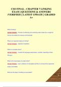
Causality (Reflective vs Formative models) → Causal assumption in psychometrics: latent variables are
assumed to cause the observed responses. This is a reflective model.
Reflective indicators
→ Latent construct → produces → item responses.
→ Example: Depression causes feelings of sadness, fatigue, and loss of interest.
→ Items are effects of the latent variable and therefore should correlate with each other.
Formative indicators
→ Items combine to form the construct; the direction of causality is reversed.
→ Example: Socio-economic status is formed by income, education, and occupation.
→ The indicators may or may not correlate, since they are not caused by one latent source.
Reflective constructs = causal source lies in the latent variable.
Formative constructs = causal source lies in the indicators themselves.
Psychological theory shapes expectations about:
Page 3
, • Distribution of the latent variable (normal, discrete, categorical).
• Relationships between items (correlations).
Statistics quantify those relationships and evaluate whether the data fit the theory. Causality
connects theory and data by specifying direction:
- latent → observed (reflective) or observed → latent (formative).
Measurement scales
• Nominal: Categories only (identity). E.g., gender 0/1, political party.
• Ordinal: Rank order but unequal intervals. E.g., Likert 0–4, severity levels.
• Interval: Equal intervals, no true zero. E.g., temperature in °C.
• Ratio: Equal intervals + absolute zero. E.g., reaction time, weight.
In psychology, we mostly deal with ordinal or interval-like variables (e.g., questionnaire scores treated
as continuous).
Lecture 2 - Interpreting Test Scores and Validity
Why “interpreting” matters
A raw test score (e.g., 4 on a procrastination scale) has no meaning by itself. We need to compare it
to a reference group (the norm sample) to know if it’s “high” or “low.” In contrast to physical traits
like weight or height, psychological variables don't have universal units.
↳ We can’t say “1 unit of extraversion = 1 kg”; units are arbitrary.
Therefore, interpretation always involves relative comparison:
o Person vs. person (who scores higher)
o Person vs. population norm (how typical or extreme a score is)
Norm Scores – Standardizing a Score
Raw score → z-score
• z-score = how many standard deviations a person’s score differs from the mean.
• Formula → z = (X – M) / SD
• M = mean of sample, SD = standard deviation
• Example (Maria, procrastination test):
o Raw score = 4, M = 2.704 SD = 1.552
o → z = (4 – 2.704)/1.552 = 0.835 ➜ Maria scores ≈ 0.84 SD above the mean → relatively
high procrastination.
z → t-score
• t-score = rescaled z-score to a distribution with M = 50, SD = 10.
• Formula → T = z × 10 + 50
• Maria’s t = 0.835 × 10 + 50 = 58.35 ➜ Her score is about 8 points above average, still ≈ 1 SD
above mean.
• Used because it avoids negative numbers and is easy to interpret (“50 = average”).
z → Percentile Rank (PR)
Page 4
Lecture notes and Tutorials
This summary is based on the lecture slides for Measurement Theory and Assessment by Pelt (2025–
2026).
Week 1
Lecture 1 - Introduction to Psychometrics
Psychological Measurement
Measurement in psychology = the assignment of numerals to psychological characteristics of individuals
according to rules.
↳ Example: “I like to go to parties” → No = 0, Yes = 1.
The characteristic refers to an underlying psychological variable or construct (e.g., extraversion,
anxiety). The rules come from a defined test procedure (e.g., self-report items, behavioural tasks,
reaction times).
Psychometrics = the science of evaluating psychological tests → concerned with test properties such
as reliability, validity, and bias.
↳ It applies to all types of psychological measurement – not only self-report but also performance-
based or behavioural measures.
Psychologists need to know whether their measurement tools are:
• Reliable → consistent across time, items, or raters.
• Valid → actually measuring what they claim to measure.
• Fair (unbiased) → not disadvantaging certain groups.
Key questions include:
➢ “Is my test valid for this purpose?”
➢ “Is it reliable enough to draw conclusions?”
➢ “Are scores comparable across groups or situations?”
Latent and Observed Variables
Many psychological constructs are latent variables – they cannot be observed directly (e.g.,
depression, intelligence). We infer them through observable indicators such as responses,
performance, or physiological measures.
• Observable variables = responses to items or tasks (e.g., “I feel sad,” number of remembered
words).
• Latent variable models use path diagrams:
o Latent variable → shown as a circle (unobservable).
o Observed items → shown as boxes.
o Arrows (→) represent the assumed causal direction from latent → observed.
Measurement error → every observed variable relates to the latent variable imperfectly.
↳ Hence, we always model an error term (in a small circle).
Page 1
,Roles of Theory, Statistics, and Causality
Theory: Psychological theory defines what should be measured and how it manifests.
o Example: ADHD theory → inattention + hyperactivity + impulsivity.
o Personality theory → Big Five (OCEAN) dimensions.
Theory guides:
1. Which latent constructs to include.
2. How to operationalize them into observable items.
3. Expectations about how items interrelate (dimensionality).
Statistics provides tools to examine individual differences in item responses. Core quantities: mean,
variance, covariance, correlation, and regression.
• Variance = spread of scores around the mean.
• Correlation = degree of standardized covariance between two variables. “How strongly are X
and Y related?”
• Covariance = indicates how much two variables change together. A positive covariance means
the variables tend to move in the same direction, while a negative covariance indicates they
move in opposite directions.
• Regression = estimation of relationships between a dependent variable and one or more
independent variables. “Can I predict Y if I know X?”
Regression models link latent and observed variables:
• Latent variable → item + error (b = strength of relationship).
Correlation does not imply causation → statistical association alone is not enough to interpret
meaning.
Skewness
Skewness tells you about the symmetry (or asymmetry) of a distribution — in other words, whether
the data are pulled to one side.
1. Positive Skew (Right-Skewed)
a. Tail on the right side
b. The right tail (higher values) is longer or fatter.
c. Most scores are low, with a few very high values pulling the mean upward.
d. Mean > Median > Mode
Example: Income, reaction times — a few people earn a lot, but most earn less.
Tip to remember:
The tail points to the direction of the skew — right tail → positive skew.
Page 2
, 2. Negative Skew (Left-Skewed)
a. Tail on the left side
b. The left tail (lower values) is longer or fatter.
c. Most scores are high, with a few low outliers pulling the mean downward.
d. Mean < Median < Mode
Example: Age at retirement — most retire around the same age, but a few retire very
early.
Symmetrical Distribution:
- No skew — looks like a bell curve (normal distribution).
- Mean = Median = Mode
Kurtosis
Kurtosis describes the "tailedness" or peakedness" of a distribution = how heavy or light the tails are
compared to a normal distribution. A normal distribution is bell-shaped, has medium tails (neither too
thick nor thin). There are two types of kurtosis:
1. Positive kurtosis
a. Very tall peak and fat tails
b. Data are clustered tightly around the mean, but with more extreme outliers
c. Indicates more risks/variability in extremes
Example: Exam scores where most people get average marks, but a few get very high or
very low.
2. Negative kurtosis
a. Flat peak and thin tails
b. Values are spread out more evenly with fewer outliers
Causality (Reflective vs Formative models) → Causal assumption in psychometrics: latent variables are
assumed to cause the observed responses. This is a reflective model.
Reflective indicators
→ Latent construct → produces → item responses.
→ Example: Depression causes feelings of sadness, fatigue, and loss of interest.
→ Items are effects of the latent variable and therefore should correlate with each other.
Formative indicators
→ Items combine to form the construct; the direction of causality is reversed.
→ Example: Socio-economic status is formed by income, education, and occupation.
→ The indicators may or may not correlate, since they are not caused by one latent source.
Reflective constructs = causal source lies in the latent variable.
Formative constructs = causal source lies in the indicators themselves.
Psychological theory shapes expectations about:
Page 3
, • Distribution of the latent variable (normal, discrete, categorical).
• Relationships between items (correlations).
Statistics quantify those relationships and evaluate whether the data fit the theory. Causality
connects theory and data by specifying direction:
- latent → observed (reflective) or observed → latent (formative).
Measurement scales
• Nominal: Categories only (identity). E.g., gender 0/1, political party.
• Ordinal: Rank order but unequal intervals. E.g., Likert 0–4, severity levels.
• Interval: Equal intervals, no true zero. E.g., temperature in °C.
• Ratio: Equal intervals + absolute zero. E.g., reaction time, weight.
In psychology, we mostly deal with ordinal or interval-like variables (e.g., questionnaire scores treated
as continuous).
Lecture 2 - Interpreting Test Scores and Validity
Why “interpreting” matters
A raw test score (e.g., 4 on a procrastination scale) has no meaning by itself. We need to compare it
to a reference group (the norm sample) to know if it’s “high” or “low.” In contrast to physical traits
like weight or height, psychological variables don't have universal units.
↳ We can’t say “1 unit of extraversion = 1 kg”; units are arbitrary.
Therefore, interpretation always involves relative comparison:
o Person vs. person (who scores higher)
o Person vs. population norm (how typical or extreme a score is)
Norm Scores – Standardizing a Score
Raw score → z-score
• z-score = how many standard deviations a person’s score differs from the mean.
• Formula → z = (X – M) / SD
• M = mean of sample, SD = standard deviation
• Example (Maria, procrastination test):
o Raw score = 4, M = 2.704 SD = 1.552
o → z = (4 – 2.704)/1.552 = 0.835 ➜ Maria scores ≈ 0.84 SD above the mean → relatively
high procrastination.
z → t-score
• t-score = rescaled z-score to a distribution with M = 50, SD = 10.
• Formula → T = z × 10 + 50
• Maria’s t = 0.835 × 10 + 50 = 58.35 ➜ Her score is about 8 points above average, still ≈ 1 SD
above mean.
• Used because it avoids negative numbers and is easy to interpret (“50 = average”).
z → Percentile Rank (PR)
Page 4