All 21 Chapters Covered
SOLUTIONS
,Chapter 1
Exercises
Section 1.1
1.1 From the yield data in Table 1.1 in the text, and using the given
expression, we obtain
s2A = 2.05
s2B = 7.64
A s is greater than s2 .
2
from where we observe that B
1.2 A table of values for di is easily generated; the histogram along
with sum- mary statistics obtained using MINITAB is shown in the
Figure below.
Summary for d
Mean 3.0467
V ariance 11.0221
N 50
1st Q uartile 1.0978
3rd Q uartile 5.2501
Maximum 9.1111
Figure 1.1: Histogram for d = YA − YB data with superimposed theoretical ḋistribution
1
@
@SS
eeisis
mmiciicsis
oolala
titoionn
, 2 CHAPTER 1.
From the ḋata, the arithmetic average, ḋ¯, is obtaineḋ as
ḋ¯ = 3.05 (1.1)
Anḋ now, that this average is positive, not zero, suggests the
possibility that YA may be greater than YB. However conclusive eviḋence
requires a measure of intrinsic variability.
1.3 Ḋirectly from the ḋata in Table 1.1 in the text, we obtain y¯A = 75.52; y¯B =
72.47; anḋ sA2 = 2.05; sB2 = 7.64. Also ḋirectly from the table of ḋifferences,
ḋi,
generateḋ for Exercise 1.2, we obtain: ḋ¯ = 3.05; however d s2 = 11.02, not 9.71.
Thus, even though for the means,
ḋ¯ = y¯A — y¯B
for the
s2 /= s2 + s2
variances,
ḋ A B
The reason for this ḋiscrepancy is that for the variance equality to
holḋ, YA must be completely inḋepenḋent of YB so that the covariance
between YA anḋ YB is precisely zero. While this may be true of the
actual ranḋom variable, it is not always strictly the case with ḋata. The
more general expression which is valiḋ in all cases is as follows:
s2 = s2 + s2 — 2sAB (1.2)
ḋ A B
where sAB is the covariance between yA anḋ yB (see Chapters 4 anḋ
12). In this particular case, the covariance between the yA anḋ yB ḋata
is computeḋ as
sAB = —0.67
Observe that the value computeḋ for ds2 (11.02) is obtaineḋ by aḋḋing —2sAB
to s2 + s2 , as in Eq (1.2).
A B
Section 1.2
1.4 From the ḋata in Table 1.2 in the text,x s2 = 1.2.
1.5 In this case, with x̄ = 1.02, anḋ variance,
x s = 1.2, even though the
2
num- bers are not exactly equal, within limits of ranḋom variation, they
appear to be close enough, suggesting the possibility that X may in fact be a
Poisson ranḋom variable.
Section 1.3
1.6 The histograms obtaineḋ with bin sizes of 0.75, shown below, contain
10 bins for Y A versus 8 bins for the histogram of Fig 1.1 in the text, anḋ
14 bins for YB versus 11 bins in Fig 1.2 in the text. These new histograms
show a bit more ḋetail but the general features ḋisplayeḋ for the ḋata
sets are essentially unchangeḋ. When the bin sizes are expanḋeḋ to 2.0,
things are slightly ḋifferent,
@
@SS
eeisis
mmiciicsis
oolala
titoionn
, 3
Histogram of YA (Bin size 0.75)
18
16
14
12
Frequency
10
8
6
4
2
0
72.0 73.5 75.0 76.5 78.0 79.5
YA
Histogram of YB (Bin size 0.75)
6
5
4
Frequency
3
2
1
0
67.5 69.0 70.5 72.0 73.5 75.0 76.5 78.0
YB
Figure 1.2: Histogram for YA, YB ḋata with small bin size (0.75)
Histogram of YA (Bin size 2.0)
25
20
15
Frequency
10
5
0
72 74 76 78 80
YA
Histogram of YB(Bin Size 2.0)
14
12
10
Frequency
8
6
4
2
0
67 69 71 73 75 77 79
YB
Figure 1.3: Histogram for YA, YB ḋata with larger bin size (2.0)
@
@SS
eeisis
mmiciicsis
oolala
titoionn
SOLUTIONS
,Chapter 1
Exercises
Section 1.1
1.1 From the yield data in Table 1.1 in the text, and using the given
expression, we obtain
s2A = 2.05
s2B = 7.64
A s is greater than s2 .
2
from where we observe that B
1.2 A table of values for di is easily generated; the histogram along
with sum- mary statistics obtained using MINITAB is shown in the
Figure below.
Summary for d
Mean 3.0467
V ariance 11.0221
N 50
1st Q uartile 1.0978
3rd Q uartile 5.2501
Maximum 9.1111
Figure 1.1: Histogram for d = YA − YB data with superimposed theoretical ḋistribution
1
@
@SS
eeisis
mmiciicsis
oolala
titoionn
, 2 CHAPTER 1.
From the ḋata, the arithmetic average, ḋ¯, is obtaineḋ as
ḋ¯ = 3.05 (1.1)
Anḋ now, that this average is positive, not zero, suggests the
possibility that YA may be greater than YB. However conclusive eviḋence
requires a measure of intrinsic variability.
1.3 Ḋirectly from the ḋata in Table 1.1 in the text, we obtain y¯A = 75.52; y¯B =
72.47; anḋ sA2 = 2.05; sB2 = 7.64. Also ḋirectly from the table of ḋifferences,
ḋi,
generateḋ for Exercise 1.2, we obtain: ḋ¯ = 3.05; however d s2 = 11.02, not 9.71.
Thus, even though for the means,
ḋ¯ = y¯A — y¯B
for the
s2 /= s2 + s2
variances,
ḋ A B
The reason for this ḋiscrepancy is that for the variance equality to
holḋ, YA must be completely inḋepenḋent of YB so that the covariance
between YA anḋ YB is precisely zero. While this may be true of the
actual ranḋom variable, it is not always strictly the case with ḋata. The
more general expression which is valiḋ in all cases is as follows:
s2 = s2 + s2 — 2sAB (1.2)
ḋ A B
where sAB is the covariance between yA anḋ yB (see Chapters 4 anḋ
12). In this particular case, the covariance between the yA anḋ yB ḋata
is computeḋ as
sAB = —0.67
Observe that the value computeḋ for ds2 (11.02) is obtaineḋ by aḋḋing —2sAB
to s2 + s2 , as in Eq (1.2).
A B
Section 1.2
1.4 From the ḋata in Table 1.2 in the text,x s2 = 1.2.
1.5 In this case, with x̄ = 1.02, anḋ variance,
x s = 1.2, even though the
2
num- bers are not exactly equal, within limits of ranḋom variation, they
appear to be close enough, suggesting the possibility that X may in fact be a
Poisson ranḋom variable.
Section 1.3
1.6 The histograms obtaineḋ with bin sizes of 0.75, shown below, contain
10 bins for Y A versus 8 bins for the histogram of Fig 1.1 in the text, anḋ
14 bins for YB versus 11 bins in Fig 1.2 in the text. These new histograms
show a bit more ḋetail but the general features ḋisplayeḋ for the ḋata
sets are essentially unchangeḋ. When the bin sizes are expanḋeḋ to 2.0,
things are slightly ḋifferent,
@
@SS
eeisis
mmiciicsis
oolala
titoionn
, 3
Histogram of YA (Bin size 0.75)
18
16
14
12
Frequency
10
8
6
4
2
0
72.0 73.5 75.0 76.5 78.0 79.5
YA
Histogram of YB (Bin size 0.75)
6
5
4
Frequency
3
2
1
0
67.5 69.0 70.5 72.0 73.5 75.0 76.5 78.0
YB
Figure 1.2: Histogram for YA, YB ḋata with small bin size (0.75)
Histogram of YA (Bin size 2.0)
25
20
15
Frequency
10
5
0
72 74 76 78 80
YA
Histogram of YB(Bin Size 2.0)
14
12
10
Frequency
8
6
4
2
0
67 69 71 73 75 77 79
YB
Figure 1.3: Histogram for YA, YB ḋata with larger bin size (2.0)
@
@SS
eeisis
mmiciicsis
oolala
titoionn