Week 2 HW: ISYE 6501
By: Kethan Anasuri
Table of Contents
1. Question 4.1
2. Question 4.2
• 1. Identifying the best value of k
• 2. Choosing the best cluster
3. Question 5.1
1. Exploratory Data Analysis
2. Grubbs test
3. Conclusion
4. Question 6.1
5. Question 6.2
1. Question 6.2.1
2. Question 6.2.2
6. References
Question 4.1
One real-life example of clustering may be applied to the retail industry. For example, grocery stores
may want to use clustering to identify which grocery items sell the most. What differentiates this from a
classification problem or a supervised learning approach stems from the fact that the groups of items that
sell the most have not been identified beforehand. Some predictors that may assist in identifying the type
of best-selling items at a grocery store include:
1. Frequency being bought
2. Item type (produce, stationery, toiletries, etc)
3. Age of consumer
4. Cost of item
The frequency and cost of items will directly go into the mathematical calculation of best-selling. However,
providing other predictors such as item type and age of consumer can better provide some context on the
people who are buying some of the best-selling their products. Having all these predictors may allow the
grocery store to tailor to their audience while also knowing which products are bringing in the most value.
Question 4.2
1. Identifying the best value of k
To identify the best value of k, we would want to examine the total distance of each data point to its cluster
center. This is done by returning the value of tot.withinss or the total value of the sum of squares within
each cluster, and comparing the values across different values of k
1
, From the elbow plot, we can see that the value at which there is marginal upgrade in increasing the amount
of clusters is at k = 3 clusters. This makes sense because when we examine the data set, we know that there
are 3 types of flowers: setosa, versicolor, and virginica. I also found it helpful to tweak the value of nstart in
the kmeans function. This is because the values of nstart will create multiple different configurations with
various random initial centroids and report the best one. If the initial random centroid is chosen poorly,
then the total distance between each data point and each cluster center will likely be larger (given smaller
amounts of clusters chosen), and it will take longer to converge.
2. Choosing the best cluster
When choosing the best cluster, it requires understanding which characteristics play the largest role in
identifying clusters. With the help of the ggplot library, I’ve decided to plot the 4 attributes against each
other on the original dataset to try and see the clusters, and the Petal Width and Petal Length seem to
contribute the largest to clustering the 3 types of flowers. Here is a representation below:
From here, we can see that the setosa flowers have petal lengths <2 cm and petal widths <0.75 cm. Next,
the the versicolor flowers have petal lengths ranging from 3 cm to ~5 cm, while their widths are ~1-1.75
2
By: Kethan Anasuri
Table of Contents
1. Question 4.1
2. Question 4.2
• 1. Identifying the best value of k
• 2. Choosing the best cluster
3. Question 5.1
1. Exploratory Data Analysis
2. Grubbs test
3. Conclusion
4. Question 6.1
5. Question 6.2
1. Question 6.2.1
2. Question 6.2.2
6. References
Question 4.1
One real-life example of clustering may be applied to the retail industry. For example, grocery stores
may want to use clustering to identify which grocery items sell the most. What differentiates this from a
classification problem or a supervised learning approach stems from the fact that the groups of items that
sell the most have not been identified beforehand. Some predictors that may assist in identifying the type
of best-selling items at a grocery store include:
1. Frequency being bought
2. Item type (produce, stationery, toiletries, etc)
3. Age of consumer
4. Cost of item
The frequency and cost of items will directly go into the mathematical calculation of best-selling. However,
providing other predictors such as item type and age of consumer can better provide some context on the
people who are buying some of the best-selling their products. Having all these predictors may allow the
grocery store to tailor to their audience while also knowing which products are bringing in the most value.
Question 4.2
1. Identifying the best value of k
To identify the best value of k, we would want to examine the total distance of each data point to its cluster
center. This is done by returning the value of tot.withinss or the total value of the sum of squares within
each cluster, and comparing the values across different values of k
1
, From the elbow plot, we can see that the value at which there is marginal upgrade in increasing the amount
of clusters is at k = 3 clusters. This makes sense because when we examine the data set, we know that there
are 3 types of flowers: setosa, versicolor, and virginica. I also found it helpful to tweak the value of nstart in
the kmeans function. This is because the values of nstart will create multiple different configurations with
various random initial centroids and report the best one. If the initial random centroid is chosen poorly,
then the total distance between each data point and each cluster center will likely be larger (given smaller
amounts of clusters chosen), and it will take longer to converge.
2. Choosing the best cluster
When choosing the best cluster, it requires understanding which characteristics play the largest role in
identifying clusters. With the help of the ggplot library, I’ve decided to plot the 4 attributes against each
other on the original dataset to try and see the clusters, and the Petal Width and Petal Length seem to
contribute the largest to clustering the 3 types of flowers. Here is a representation below:
From here, we can see that the setosa flowers have petal lengths <2 cm and petal widths <0.75 cm. Next,
the the versicolor flowers have petal lengths ranging from 3 cm to ~5 cm, while their widths are ~1-1.75
2