ALL 8 CHAPTERS COVERED
SOLUTIONS MANUAL
, Chapter 1
CHAPTER 1
SECTION 1.2
1.2.1:
The inequality T∞ ≥ log n in the statement of Prop. 2.1 is replaced by the inequality T∞ ≥ logB n,
where log B stands for the base B logarithm. The proof is similar with the proof of Prop. 2.1. We
show by induction on k, that tj ≥ logB k for every node j depending on k inputs, and for every
schedule. The claim is clearly true if k = 1. Assume that the claim is true for every k smaller than
some k0 and consider a node j that depends on k0 + 1 inputs. Since j has at most B predecessors,
it has a predecessor ℓ that depends on at least ⌈(k0 + 1)/B⌉ inputs. Then, using the induction
hypothesis,
» ¼ µ 
k0 + 1 k0 + 1
tj ≥ tℓ + 1 ≥ logB + 1 ≥ logB + 1 = logB (k0 + 1),
B B
which completes the induction.
1.2.2:
Here we need to assume that a particular algorithm has been fixed and that T ∗ (n) is its serial
execution time. We assume that a fraction f of the algorithm is inherently serial. This part
requires fT ∗ (n) time no matter how many processors we try to use. The remaining fraction, which
is 1 − f, needs at least (1 − f )T ∗ (n)/p time, when p processors are available. Thus, Tp (n) ≥
¡ ¢
f + (1 − f)/p T ∗ (n), which yields
T ∗ (n) 1 1
Sp (n) = ≤ ≤ .
Tp (n) f + (1 − f)/p f
1.2.3:
(a) The main idea here is to divide and conquer. We start by considering the case where n is a
power of 2. If n = 1, there is nothing to be done and the problem is solved in zero time using
1
, Chapter 1
zero processors. Assume that have already constructed a parallel algorithm that solves the prefix
problem for some n which is a power of 2, in time T (n) using p(n) processors. We now construct
an algorithm that solves the same problem when n is replaced by 2n. We use the already available
algorithm to compute all of the quantities ki=1 ai , k = 1, 2, . . . , n, and ki=n+1 ai , k = n + 1, . . . , 2n.
Q Q
This amounts to solving two prefix problems, each one involving n numbers. This can be done in
Qk
parallel, in time T (n) using 2p(n) processors. We then multiply each one of the numbers i=n+1 ai ,
k = n + 1, . . . , 2n, by ni=1 ai , and this completes the desired computation. This last stage can be
Q
performed in a single stage, using n processors.
The above described recursive definition provides us with a prefix algorithm for every value of n
which is a power of 2. Its time and processor requirements are given by
T (2n) = T (n) + 1,
n o
p(2n) = max 2p(n), n .
Using the facts T (1) = 0 and p(1) = 0, an easy inductive argument shows that T (n) = log n and
p(n) = n/2.
The case where n is not a power of 2 cannot be any harder than the case where n is replaced by
the larger number 2⌈log n⌉ . Since the latter number is a power of 2, we obtain
³ ´ ³ ´
T (n) ≤ T 2⌈log n⌉ = log 2⌈log n⌉ = ⌈log n⌉,
and
³ ´
p(n) ≤ p 2⌈log n⌉ = 2⌈log n⌉−1 < 2logn = n.
(b) The algorithm is identical with part (a) except that each scalar multiplication is replaced by a
multiplication of two m × m matrices. Each such multiplication can be performed in time O(log m)
using O(m3 ) processors, as opposed to unit time with one processor. Thus, the time of the algorithm
is O(log m · log n), using O(nm3 ) processors.
(c) The solution of the difference equation x(t + 1) = A(t)x(t) + u(t) is given by
h n−1
Y i n−1 h n−1
X Y i
x(n) = A(j) x(0) + A(j) u(i).
j=0 i=0 j=i+1
Qn−1
We use the algorithm of part (b) to compute the matrix products j=i A(j), for i = 0, 1, . . . , n − 1.
This takes O(log m · log n) time. We then multiply each such product with the corresponding vector
u(i) or x(0) [this can be done in parallel, in O(log m) time], and then add the results [this can be
done in parallel in O(log n) time]. We conclude that the overall time is O(log m · log n) + O(log m) +
O(log n) = O(log m · log n).
2
, Chapter 1
1.2.4:
We represent k in the form
⌊log k⌋
X
k= bi 2i ,
i=0
where each bi belongs to the set {0, 1}. (In particular, the coefficients bi are the entries in the binary
representation of k.) Then,
⌊log k⌋
Y i
Ak = Abi 2 . (1)
i=0
⌊log k⌋
We compute the matrices A2 , A4 , . . . , A2 by successive squaring, and then carry out the matrix
multiplications in Eq. (1). It is seen that this algorithm consists of at most 2⌊log k⌋ successive matrix
multiplications and the total parallel time is O(log n · log k), using O(n3 ) processors.
1.2.5:
(a) Notice that " # " #" #
x(t + 1) a(t) b(t) x(t)
= .
x(t) 1 0 x(t − 1)
We define " #
a(t) b(t)
A(t) = ,
1 0
to obtain " # " #
x(n) x(0)
= A(n − 1)A(n − 2) · · · A(1)A(0) . (1)
x(n − 1) x(−1)
This reduces the problem to the evaluation of the product of n matrices of dimensions 2 × 2, which
can be done in O(log n) time, using O(n) processors [cf. Exercise 1.2.3(b)].
(b) Similarly with Eq. (1), we have
" # " #
x(n) x(1)
=D , (2)
x(n − 1) x(0)
where D = A(n − 1)A(n − 2) · · · A(1). This is a linear system of two equations in the four variables
x(0), x(1), x(n − 1), x(n). Furthermore, the coefficients of these equations can be computed in
O(log n) time as in part (a). We fix the values of x(0) and x(n − 1) as prescribed, and we solve for
the remaining two variables using Cramer’s rule (which takes only a constant number of arithmetic
operations). This would be the end of the solution, except for the possibility that the system of
equations being solved is singular (in which case Cramer’s rule breaks down), and we must ensure
that this is not the case. If the system is singular, then either there exists no solution for x(1)
and x(n), or there exist several solutions. The first case is excluded because we have assumed
3
, Chapter 1
the existence of a sequence x(0), . . . , x(n) compatible with the boundary conditions on x(0) and
x(n − 1), and the values of x(1), x(n) corresponding to that sequence must also satisfy Eq. (2).
¡ ¢ ¡ ¢
Suppose now that Eq. (2) has two distinct solutions x1 (1), x1 (n) and x2 (1), x2 (n) . Consider the
¡ ¢ ¡ ¢
original difference equation, with the two different initial conditions x(0), x1 (1) and x(0), x2 (1) .
By solving the difference equation we obtain two different sequences, both of which satisfy Eq. (2)
and both of which have the prescribed values of x(0) and x(n − 1). This contradicts the uniqueness
assumption in the statement of the problem and concludes the proof.
1.2.6:
We first compute x2 , x3 , . . . , xn−1 , xn , and then form the inner product of the vectors
(1, x, x2 , . . . , xn ) and (a0 , a1 , . . . , an ). The first stage is no harder than the prefix problem of Ex-
ercise 1.2.3(a). (Using the notation of Exercise 1.2.3, we are dealing with the special case where
ai = x for each i.) Thus, the first stage can be performed in O(log n) time. The inner product
evaluation in the second stage can also be done in O(log n) time. (A better algorithm can be found
in [MuP73]).
1.2.7:
(a) Notice that the graph in part (a) of the figure is a subgraph of the dependency graph of Fig.
1.2.12. In this subgraph, every two nodes are neighbors and, therefore, different colors have to be
assigned to them. Thus, four colors are necessary.
(b) See part (b) of the figure.
(c) Assign to each processor a different “column” of the graph. Note: The result of part (c) would
not be correct if the graph had more than four rows.
SECTION 1.3
1.3.1:
Let kA and kB be as in the hint. Then, based on the rules of the protocol, the pair (kA , kB ) changes
periodically as shown in the figure. (To show that this figure is correct, one must argue that at
state (1, 1), A cannot receive a 0, at state (1, 0), which would move the state to (0, 1), B cannot
4
, Chapter 1
Figure For Exercise 1.2.7.
receive a 1, etc.). B stores a packet numbered 0 when the state changes from (1, 1) to (1, 0), and
stores a packet numbered 1 when the state changes from (0, 0) to (0, 1). Thus, B alternates between
storing a packet numbered 0 and a packet numbered 1. It follows that packets are received in order.
Furthermore each packet is received only once, because upon reception of a 0 following a 1, B will
discard all subsequent 0’s and will only accept the first subsequent 1 (a similar argument holds also
with the roles of 0 and 1 reversed). Finally, each packet will eventually be received by B, that is, the
system cannot stop at some state (assuming an infinite packet supply at A). To see this, note that
at state (1, 1), A keeps transmitting packet 0 (after a timeout of ∆) up to the time A receices a 0
from B. Therefore, B will eventually receive one of these 0’s switching the state to (1, 0). Similarly,
at state (1, 0), B keeps transmitting 0’s in response to the received 0’s, so eventually one of these 0’s
will be received by A, switching the state to (0, 0), and the process will be repeated with the roles
of 0 and 1 reversed.
1.3.2:
(a) We claim that the following algorithm completes a multinode broadcast in p − 1 time units.
At the first time unit, each node sends its packet to all its neighbors. At every time unit after
the first, each processor i considers each of its incident links (i, j). If i has received a packet that
it has neither sent already to j, nor it has yet received from j, then i sends such a packet on link
(i, j). If i does not have such a packet, it sends nothing on (i, j).
For each link (i, j), let T (i, j) be the set of nodes whose unique simple walk to i on the tree passes
through j, and let n(i, j) be the number of nodes in the set T (i, j). We claim that in the preceding
algorithm, each node i receives from each neighbor j a packet from one of the nodes of T (i, j) at
5
, Chapter 1
Figure For Exercise 1.3.1. State transition diagram for the stop-and-
wait protocol.
each of the time units 1, 2, . . . , n(i, j), and as a result, the multinode broadcast is completed in
max(i,j) n(i, j) = p − 1 time units.
We prove our claim by induction. It is true for all links (i, j) with n(i, j) = 1, since all nodes
receive the packets of their neighbors at the first time unit. Assuming that the claim is true for all
links (i, j) with n(i, j) = k, we will show that the claim is true for all (i, j) with n(i, j) = k + 1.
Indeed let (i, j) be such that n(i, j) = k + 1 and let j1 , j2 , . . . , jm be the neighbors of j other than i.
Then we have
T (i, j) = (i, j) ∪ ∪m
¡ ¢
v=1 T (j, jv )
and therefore
m
X
n(i, j) = 1 + n(j, jv ).
v=1
Node i receives from j the packet of j at the first time unit. By the induction hypothesis, j has
received at least t packets by the end of t time units, where t = 1, 2, . . . , m
P
v=1 n(j, jv ). Therefore, j
has a packet to send to i from some node in ∪m v=1 T (j, jv ) ⊂ T (i, j) at each time unit t = 2, 3, . . . , 1 +
Pm
v=1 n(i, jv ). By the rules of the algorithm, i receives such a packet from j at each of these time
units, and the induction proof is complete.
(b) Let T1 and T2 be the subtrees rooted at the two neighbors of the root node. In a total exchange,
all of the Θ(p2 ) packets originating at nodes of T1 and destined for nodes of T2 must be transmitted
by the root node. Therefore any total exchange algorithm requires Ω(p2 ) time. We can also perform
a total exchange by carrying out p successive multinode broadcasts requiring p(p − 1) time units
as per part (a). Therefore an optimal total exchange requires Θ(p2 ) time units. [The alternative
algorithm, based on the mapping of a unidirectional ring on the binary balanced tree (cf. Fig. 1.3.29)
6
, Chapter 1
is somewhat slower, but also achieves the optimal order of time for a total exchange.]
1.3.3:
Let (00 · · · 0) be the identity of node A and (10 · · · 0) be the identity of node B. The identity of an
adjacent node of A, say C, has an identity with one unity bit, say the ith from the left, and all other
bits zero. If i = 1, then C = B and node A is the only node in SB that is a neighbor of C. If i > 1,
then the node with bits 1 and i unity is the only node in SB that is a neighbor of C.
1.3.4:
(a) Consider a particular direction for traversing the cycle. The identity of each successive node of
the cycle differs from the one of its predecessor node by a single bit, so going from one node to the
next on the cycle corresponds to reversing a single bit. After traversing the cycle once, ending up at
the starting node, each bit must have been reversed an even number of times. Therefore, the total
number of bit reversals, which is the number of nodes in the cycle, is even.
(b) For p even, the ring can be mapped into a 2 × 2d−1 mesh, which in turn can be mapped into a
d-cube. If p is odd and a mapping of the p-node ring into the d-cube existed, we would have a cycle
on the d-cube with an odd number of nodes contradicting part (a).
1.3.5:
See the figure.
Figure Solution of Exercise 1.3.5.
7
, Chapter 1
1.3.6:
Follow the given hint. In the first phase, each node (x1 , x2 , . . . , xd ) sends to each node of the form
(x1 , y2 , . . . , yd ) the p1/d packets destined for nodes (y1 , y2 , . . . , yd ), where y1 ranges over 1, 2, . . . , p1/d .
This involves p1/d total exchanges in (d − 1)-dimensional meshes with p(d−1)/d nodes each. By the
¡ ¢
induction hypothesis, each of these total exchanges takes time O (p(d−1)/d )d/(d−1) = O(p), for a total
¡ ¢
of p1/d O(p) = O p(d+1)/d time. At the end of phase one, each node (x1 , x2 , . . . , xd ) has p(d−1)/d p1/d
packets, which must be distributed to the p1/d nodes obtained by fixing x2 , x3 , . . . , xd , that is, nodes
(y1 , x2 , . . . , xd ) where y1 = 1, 2, . . . , p1/d . This can be done with p(d−1)/d total exchanges within one-
¡ ¢
dimensional arrays with p1/d nodes. Each total exchange takes O (p1/d )2 time (by the results of
¡ ¢ ¡ ¢
Section 1.3.4), for a total of p(d−1)/d O p2/d = O p(d+1)/d time.
1.3.7:
See the hint.
1.3.8:
Without loss of generality, assume that the two node identities differ in the rightmost bit. Let C1 (or
C2 ) be the (d − 1)-cubes of nodes whose identities have zero (or one, respectively) as the rightmost
bit. Consider the following algorithm: at the first time unit, each node starts an optimal single
node broadcast of its own packet within its own (d − 1)-cube (either C1 or C2 ), and also sends its
own packet to the other node. At the second time unit, each node starts an optimal single node
broadcast of the other node’s packet within its own (d − 1)-cube (and using the same tree as for the
first single node broadcast). The single node broadcasts takes d − 1 time units each, and can be
pipelined because they start one time unit apart and they use the same tree. Therefore the second
single node broadcast is completed at time d, at which time the two-node broadcast is accomplished.
1.3.9:
(a) Consider the algorithm of the hint, where each node receiving a packet not destined for itself,
transmits the packet at the next time unit on the next link of the path to the packet’s destination.
This algorithm accomplishes the single node scatter in p − 1 time units. There is no faster algorithm
for single node scatter, since s has p − 1 packets to transmit, and can transmit at most one per time
unit.
8
, Chapter 1
(b) Consider the algorithm of the hint, where each node receiving a packet not destined for itself,
transmits the packet at the next time unit on the next link of the path to the packet’s destination.
Then s starts transmitting its last packet to the subtree Ti at time Ni − 1, and all nodes receive
their packet at time Ni . (To see the latter, note that all packets destined for the nodes of Ti
that are k links away from s are sent before time Ni − k, and each of these packets completes its
journey in exactly k time units.) Therefore all packets are received at their respective destinations
in max{N1 , N2 , . . . , Nr } time units.
(c) We will assume without loss of generality that s = (00 · · · 0) in what follows. To construct a
spanning tree T with the desired properties, let us consider the equivalence classes Rkn introduced
in Section 1.3.4 in connection with the multinode broadcast problem. As in Section 1.3.4, we order
the classes as
(00 · · · 0)R11 R21 · · · R2n2 · · · Rk1 · · · Rknk · · · R(d−2)1 · · · R(d−2)nd−2 R(d−1)1 (11 · · · 1)
and we consider the numbers n(t) and m(t) for each identity t, but for the moment, we leave the
choice of the first element in each class Rkn unspecified. We denote by mkn the number m(t) of the
first element t of Rkn and we note that this number depends only on Rkn and not on the choice of
the first element within Rkn .
We say that class R(k−1)n′ is compatible with class Rkn if R(k−1)n′ has d elements (node identities)
and there exist identities t′ ∈ R(k−1)n′ and t ∈ Rkn such that t′ is obtained from t by changing some
unity bit of t to a zero. Since the elements of R(k−1)n′ and Rkn are obtained by left shifting the bits
of t′ and t, respectively, it is seen that for every element x′ of R(k−1)n′ there is an element x of Rkn
such that x′ is obtained from x by changing one of its unity bits to a zero. The reverse is also true,
namely that for every element x of Rkn there is an element x′ of R(k−1)n′ such that x is obtained
from x′ by changing one of its zero bits to unity. An important fact for the subsequent spanning tree
construction is that for every class Rkn with 2 ≤ k ≤ d − 1, there exists a compatible class R(k−1)n′ .
Such a class can be obtained as follows: take any identity t ∈ Rkn whose rightmost bit is a one and
its leftmost bit is a zero. Let σ be a string of consecutive zeros with maximal number of bits and
let t′ be the identity obtained from t by changing to zero the unity bit immediately to the right of
σ. [For example, if t = (0010011) then t′ = (0010001) or t′ = (0000011), and if t = (0010001) then
t′ = (0010000).] Then the equivalence class of t′ is compatible with Rkn because it has d elements
[t′ 6= (00 · · · 0) and t′ contains a unique substring of consecutive zeros with maximal number of bits,
so it cannot be replicated by left rotation of less than d bits].
The spanning tree T with the desired properties is constructed sequentially by adding links
incident to elements of the classes Rkn as follows (see the figure):
Initially T contains no links. We choose arbitrarily the first element of class R11 and we add
9
SOLUTIONS MANUAL
, Chapter 1
CHAPTER 1
SECTION 1.2
1.2.1:
The inequality T∞ ≥ log n in the statement of Prop. 2.1 is replaced by the inequality T∞ ≥ logB n,
where log B stands for the base B logarithm. The proof is similar with the proof of Prop. 2.1. We
show by induction on k, that tj ≥ logB k for every node j depending on k inputs, and for every
schedule. The claim is clearly true if k = 1. Assume that the claim is true for every k smaller than
some k0 and consider a node j that depends on k0 + 1 inputs. Since j has at most B predecessors,
it has a predecessor ℓ that depends on at least ⌈(k0 + 1)/B⌉ inputs. Then, using the induction
hypothesis,
» ¼ µ 
k0 + 1 k0 + 1
tj ≥ tℓ + 1 ≥ logB + 1 ≥ logB + 1 = logB (k0 + 1),
B B
which completes the induction.
1.2.2:
Here we need to assume that a particular algorithm has been fixed and that T ∗ (n) is its serial
execution time. We assume that a fraction f of the algorithm is inherently serial. This part
requires fT ∗ (n) time no matter how many processors we try to use. The remaining fraction, which
is 1 − f, needs at least (1 − f )T ∗ (n)/p time, when p processors are available. Thus, Tp (n) ≥
¡ ¢
f + (1 − f)/p T ∗ (n), which yields
T ∗ (n) 1 1
Sp (n) = ≤ ≤ .
Tp (n) f + (1 − f)/p f
1.2.3:
(a) The main idea here is to divide and conquer. We start by considering the case where n is a
power of 2. If n = 1, there is nothing to be done and the problem is solved in zero time using
1
, Chapter 1
zero processors. Assume that have already constructed a parallel algorithm that solves the prefix
problem for some n which is a power of 2, in time T (n) using p(n) processors. We now construct
an algorithm that solves the same problem when n is replaced by 2n. We use the already available
algorithm to compute all of the quantities ki=1 ai , k = 1, 2, . . . , n, and ki=n+1 ai , k = n + 1, . . . , 2n.
Q Q
This amounts to solving two prefix problems, each one involving n numbers. This can be done in
Qk
parallel, in time T (n) using 2p(n) processors. We then multiply each one of the numbers i=n+1 ai ,
k = n + 1, . . . , 2n, by ni=1 ai , and this completes the desired computation. This last stage can be
Q
performed in a single stage, using n processors.
The above described recursive definition provides us with a prefix algorithm for every value of n
which is a power of 2. Its time and processor requirements are given by
T (2n) = T (n) + 1,
n o
p(2n) = max 2p(n), n .
Using the facts T (1) = 0 and p(1) = 0, an easy inductive argument shows that T (n) = log n and
p(n) = n/2.
The case where n is not a power of 2 cannot be any harder than the case where n is replaced by
the larger number 2⌈log n⌉ . Since the latter number is a power of 2, we obtain
³ ´ ³ ´
T (n) ≤ T 2⌈log n⌉ = log 2⌈log n⌉ = ⌈log n⌉,
and
³ ´
p(n) ≤ p 2⌈log n⌉ = 2⌈log n⌉−1 < 2logn = n.
(b) The algorithm is identical with part (a) except that each scalar multiplication is replaced by a
multiplication of two m × m matrices. Each such multiplication can be performed in time O(log m)
using O(m3 ) processors, as opposed to unit time with one processor. Thus, the time of the algorithm
is O(log m · log n), using O(nm3 ) processors.
(c) The solution of the difference equation x(t + 1) = A(t)x(t) + u(t) is given by
h n−1
Y i n−1 h n−1
X Y i
x(n) = A(j) x(0) + A(j) u(i).
j=0 i=0 j=i+1
Qn−1
We use the algorithm of part (b) to compute the matrix products j=i A(j), for i = 0, 1, . . . , n − 1.
This takes O(log m · log n) time. We then multiply each such product with the corresponding vector
u(i) or x(0) [this can be done in parallel, in O(log m) time], and then add the results [this can be
done in parallel in O(log n) time]. We conclude that the overall time is O(log m · log n) + O(log m) +
O(log n) = O(log m · log n).
2
, Chapter 1
1.2.4:
We represent k in the form
⌊log k⌋
X
k= bi 2i ,
i=0
where each bi belongs to the set {0, 1}. (In particular, the coefficients bi are the entries in the binary
representation of k.) Then,
⌊log k⌋
Y i
Ak = Abi 2 . (1)
i=0
⌊log k⌋
We compute the matrices A2 , A4 , . . . , A2 by successive squaring, and then carry out the matrix
multiplications in Eq. (1). It is seen that this algorithm consists of at most 2⌊log k⌋ successive matrix
multiplications and the total parallel time is O(log n · log k), using O(n3 ) processors.
1.2.5:
(a) Notice that " # " #" #
x(t + 1) a(t) b(t) x(t)
= .
x(t) 1 0 x(t − 1)
We define " #
a(t) b(t)
A(t) = ,
1 0
to obtain " # " #
x(n) x(0)
= A(n − 1)A(n − 2) · · · A(1)A(0) . (1)
x(n − 1) x(−1)
This reduces the problem to the evaluation of the product of n matrices of dimensions 2 × 2, which
can be done in O(log n) time, using O(n) processors [cf. Exercise 1.2.3(b)].
(b) Similarly with Eq. (1), we have
" # " #
x(n) x(1)
=D , (2)
x(n − 1) x(0)
where D = A(n − 1)A(n − 2) · · · A(1). This is a linear system of two equations in the four variables
x(0), x(1), x(n − 1), x(n). Furthermore, the coefficients of these equations can be computed in
O(log n) time as in part (a). We fix the values of x(0) and x(n − 1) as prescribed, and we solve for
the remaining two variables using Cramer’s rule (which takes only a constant number of arithmetic
operations). This would be the end of the solution, except for the possibility that the system of
equations being solved is singular (in which case Cramer’s rule breaks down), and we must ensure
that this is not the case. If the system is singular, then either there exists no solution for x(1)
and x(n), or there exist several solutions. The first case is excluded because we have assumed
3
, Chapter 1
the existence of a sequence x(0), . . . , x(n) compatible with the boundary conditions on x(0) and
x(n − 1), and the values of x(1), x(n) corresponding to that sequence must also satisfy Eq. (2).
¡ ¢ ¡ ¢
Suppose now that Eq. (2) has two distinct solutions x1 (1), x1 (n) and x2 (1), x2 (n) . Consider the
¡ ¢ ¡ ¢
original difference equation, with the two different initial conditions x(0), x1 (1) and x(0), x2 (1) .
By solving the difference equation we obtain two different sequences, both of which satisfy Eq. (2)
and both of which have the prescribed values of x(0) and x(n − 1). This contradicts the uniqueness
assumption in the statement of the problem and concludes the proof.
1.2.6:
We first compute x2 , x3 , . . . , xn−1 , xn , and then form the inner product of the vectors
(1, x, x2 , . . . , xn ) and (a0 , a1 , . . . , an ). The first stage is no harder than the prefix problem of Ex-
ercise 1.2.3(a). (Using the notation of Exercise 1.2.3, we are dealing with the special case where
ai = x for each i.) Thus, the first stage can be performed in O(log n) time. The inner product
evaluation in the second stage can also be done in O(log n) time. (A better algorithm can be found
in [MuP73]).
1.2.7:
(a) Notice that the graph in part (a) of the figure is a subgraph of the dependency graph of Fig.
1.2.12. In this subgraph, every two nodes are neighbors and, therefore, different colors have to be
assigned to them. Thus, four colors are necessary.
(b) See part (b) of the figure.
(c) Assign to each processor a different “column” of the graph. Note: The result of part (c) would
not be correct if the graph had more than four rows.
SECTION 1.3
1.3.1:
Let kA and kB be as in the hint. Then, based on the rules of the protocol, the pair (kA , kB ) changes
periodically as shown in the figure. (To show that this figure is correct, one must argue that at
state (1, 1), A cannot receive a 0, at state (1, 0), which would move the state to (0, 1), B cannot
4
, Chapter 1
Figure For Exercise 1.2.7.
receive a 1, etc.). B stores a packet numbered 0 when the state changes from (1, 1) to (1, 0), and
stores a packet numbered 1 when the state changes from (0, 0) to (0, 1). Thus, B alternates between
storing a packet numbered 0 and a packet numbered 1. It follows that packets are received in order.
Furthermore each packet is received only once, because upon reception of a 0 following a 1, B will
discard all subsequent 0’s and will only accept the first subsequent 1 (a similar argument holds also
with the roles of 0 and 1 reversed). Finally, each packet will eventually be received by B, that is, the
system cannot stop at some state (assuming an infinite packet supply at A). To see this, note that
at state (1, 1), A keeps transmitting packet 0 (after a timeout of ∆) up to the time A receices a 0
from B. Therefore, B will eventually receive one of these 0’s switching the state to (1, 0). Similarly,
at state (1, 0), B keeps transmitting 0’s in response to the received 0’s, so eventually one of these 0’s
will be received by A, switching the state to (0, 0), and the process will be repeated with the roles
of 0 and 1 reversed.
1.3.2:
(a) We claim that the following algorithm completes a multinode broadcast in p − 1 time units.
At the first time unit, each node sends its packet to all its neighbors. At every time unit after
the first, each processor i considers each of its incident links (i, j). If i has received a packet that
it has neither sent already to j, nor it has yet received from j, then i sends such a packet on link
(i, j). If i does not have such a packet, it sends nothing on (i, j).
For each link (i, j), let T (i, j) be the set of nodes whose unique simple walk to i on the tree passes
through j, and let n(i, j) be the number of nodes in the set T (i, j). We claim that in the preceding
algorithm, each node i receives from each neighbor j a packet from one of the nodes of T (i, j) at
5
, Chapter 1
Figure For Exercise 1.3.1. State transition diagram for the stop-and-
wait protocol.
each of the time units 1, 2, . . . , n(i, j), and as a result, the multinode broadcast is completed in
max(i,j) n(i, j) = p − 1 time units.
We prove our claim by induction. It is true for all links (i, j) with n(i, j) = 1, since all nodes
receive the packets of their neighbors at the first time unit. Assuming that the claim is true for all
links (i, j) with n(i, j) = k, we will show that the claim is true for all (i, j) with n(i, j) = k + 1.
Indeed let (i, j) be such that n(i, j) = k + 1 and let j1 , j2 , . . . , jm be the neighbors of j other than i.
Then we have
T (i, j) = (i, j) ∪ ∪m
¡ ¢
v=1 T (j, jv )
and therefore
m
X
n(i, j) = 1 + n(j, jv ).
v=1
Node i receives from j the packet of j at the first time unit. By the induction hypothesis, j has
received at least t packets by the end of t time units, where t = 1, 2, . . . , m
P
v=1 n(j, jv ). Therefore, j
has a packet to send to i from some node in ∪m v=1 T (j, jv ) ⊂ T (i, j) at each time unit t = 2, 3, . . . , 1 +
Pm
v=1 n(i, jv ). By the rules of the algorithm, i receives such a packet from j at each of these time
units, and the induction proof is complete.
(b) Let T1 and T2 be the subtrees rooted at the two neighbors of the root node. In a total exchange,
all of the Θ(p2 ) packets originating at nodes of T1 and destined for nodes of T2 must be transmitted
by the root node. Therefore any total exchange algorithm requires Ω(p2 ) time. We can also perform
a total exchange by carrying out p successive multinode broadcasts requiring p(p − 1) time units
as per part (a). Therefore an optimal total exchange requires Θ(p2 ) time units. [The alternative
algorithm, based on the mapping of a unidirectional ring on the binary balanced tree (cf. Fig. 1.3.29)
6
, Chapter 1
is somewhat slower, but also achieves the optimal order of time for a total exchange.]
1.3.3:
Let (00 · · · 0) be the identity of node A and (10 · · · 0) be the identity of node B. The identity of an
adjacent node of A, say C, has an identity with one unity bit, say the ith from the left, and all other
bits zero. If i = 1, then C = B and node A is the only node in SB that is a neighbor of C. If i > 1,
then the node with bits 1 and i unity is the only node in SB that is a neighbor of C.
1.3.4:
(a) Consider a particular direction for traversing the cycle. The identity of each successive node of
the cycle differs from the one of its predecessor node by a single bit, so going from one node to the
next on the cycle corresponds to reversing a single bit. After traversing the cycle once, ending up at
the starting node, each bit must have been reversed an even number of times. Therefore, the total
number of bit reversals, which is the number of nodes in the cycle, is even.
(b) For p even, the ring can be mapped into a 2 × 2d−1 mesh, which in turn can be mapped into a
d-cube. If p is odd and a mapping of the p-node ring into the d-cube existed, we would have a cycle
on the d-cube with an odd number of nodes contradicting part (a).
1.3.5:
See the figure.
Figure Solution of Exercise 1.3.5.
7
, Chapter 1
1.3.6:
Follow the given hint. In the first phase, each node (x1 , x2 , . . . , xd ) sends to each node of the form
(x1 , y2 , . . . , yd ) the p1/d packets destined for nodes (y1 , y2 , . . . , yd ), where y1 ranges over 1, 2, . . . , p1/d .
This involves p1/d total exchanges in (d − 1)-dimensional meshes with p(d−1)/d nodes each. By the
¡ ¢
induction hypothesis, each of these total exchanges takes time O (p(d−1)/d )d/(d−1) = O(p), for a total
¡ ¢
of p1/d O(p) = O p(d+1)/d time. At the end of phase one, each node (x1 , x2 , . . . , xd ) has p(d−1)/d p1/d
packets, which must be distributed to the p1/d nodes obtained by fixing x2 , x3 , . . . , xd , that is, nodes
(y1 , x2 , . . . , xd ) where y1 = 1, 2, . . . , p1/d . This can be done with p(d−1)/d total exchanges within one-
¡ ¢
dimensional arrays with p1/d nodes. Each total exchange takes O (p1/d )2 time (by the results of
¡ ¢ ¡ ¢
Section 1.3.4), for a total of p(d−1)/d O p2/d = O p(d+1)/d time.
1.3.7:
See the hint.
1.3.8:
Without loss of generality, assume that the two node identities differ in the rightmost bit. Let C1 (or
C2 ) be the (d − 1)-cubes of nodes whose identities have zero (or one, respectively) as the rightmost
bit. Consider the following algorithm: at the first time unit, each node starts an optimal single
node broadcast of its own packet within its own (d − 1)-cube (either C1 or C2 ), and also sends its
own packet to the other node. At the second time unit, each node starts an optimal single node
broadcast of the other node’s packet within its own (d − 1)-cube (and using the same tree as for the
first single node broadcast). The single node broadcasts takes d − 1 time units each, and can be
pipelined because they start one time unit apart and they use the same tree. Therefore the second
single node broadcast is completed at time d, at which time the two-node broadcast is accomplished.
1.3.9:
(a) Consider the algorithm of the hint, where each node receiving a packet not destined for itself,
transmits the packet at the next time unit on the next link of the path to the packet’s destination.
This algorithm accomplishes the single node scatter in p − 1 time units. There is no faster algorithm
for single node scatter, since s has p − 1 packets to transmit, and can transmit at most one per time
unit.
8
, Chapter 1
(b) Consider the algorithm of the hint, where each node receiving a packet not destined for itself,
transmits the packet at the next time unit on the next link of the path to the packet’s destination.
Then s starts transmitting its last packet to the subtree Ti at time Ni − 1, and all nodes receive
their packet at time Ni . (To see the latter, note that all packets destined for the nodes of Ti
that are k links away from s are sent before time Ni − k, and each of these packets completes its
journey in exactly k time units.) Therefore all packets are received at their respective destinations
in max{N1 , N2 , . . . , Nr } time units.
(c) We will assume without loss of generality that s = (00 · · · 0) in what follows. To construct a
spanning tree T with the desired properties, let us consider the equivalence classes Rkn introduced
in Section 1.3.4 in connection with the multinode broadcast problem. As in Section 1.3.4, we order
the classes as
(00 · · · 0)R11 R21 · · · R2n2 · · · Rk1 · · · Rknk · · · R(d−2)1 · · · R(d−2)nd−2 R(d−1)1 (11 · · · 1)
and we consider the numbers n(t) and m(t) for each identity t, but for the moment, we leave the
choice of the first element in each class Rkn unspecified. We denote by mkn the number m(t) of the
first element t of Rkn and we note that this number depends only on Rkn and not on the choice of
the first element within Rkn .
We say that class R(k−1)n′ is compatible with class Rkn if R(k−1)n′ has d elements (node identities)
and there exist identities t′ ∈ R(k−1)n′ and t ∈ Rkn such that t′ is obtained from t by changing some
unity bit of t to a zero. Since the elements of R(k−1)n′ and Rkn are obtained by left shifting the bits
of t′ and t, respectively, it is seen that for every element x′ of R(k−1)n′ there is an element x of Rkn
such that x′ is obtained from x by changing one of its unity bits to a zero. The reverse is also true,
namely that for every element x of Rkn there is an element x′ of R(k−1)n′ such that x is obtained
from x′ by changing one of its zero bits to unity. An important fact for the subsequent spanning tree
construction is that for every class Rkn with 2 ≤ k ≤ d − 1, there exists a compatible class R(k−1)n′ .
Such a class can be obtained as follows: take any identity t ∈ Rkn whose rightmost bit is a one and
its leftmost bit is a zero. Let σ be a string of consecutive zeros with maximal number of bits and
let t′ be the identity obtained from t by changing to zero the unity bit immediately to the right of
σ. [For example, if t = (0010011) then t′ = (0010001) or t′ = (0000011), and if t = (0010001) then
t′ = (0010000).] Then the equivalence class of t′ is compatible with Rkn because it has d elements
[t′ 6= (00 · · · 0) and t′ contains a unique substring of consecutive zeros with maximal number of bits,
so it cannot be replicated by left rotation of less than d bits].
The spanning tree T with the desired properties is constructed sequentially by adding links
incident to elements of the classes Rkn as follows (see the figure):
Initially T contains no links. We choose arbitrarily the first element of class R11 and we add
9