GENERAL MATHS BOUND REFERENCE
Chapter 1
Types of Data
Univariate Data → one variable (eg. height, eye colour, number of siblings, score on a maths test)
• Numerical (discrete/continuous) → quantitative data that can be counted or measured
- Discrete → numerical data that only consists of a set of fixed values within a range (eg. whole numbers)
- Continuous → numerical data that can consist of any value within a range (eg. whole numbers & decimals)
• Categorical → qualitative data that can be organised into categories or groups
- Nominal → categorical data that cannot be sorted into a logical ordered list or hierarchy (eg. type of bread)
- Ordinal → categorical data that can be ordered into a logical ordered list or hierarchy (eg. drink size)
Exercise Example: classify the following variables as either categorical or numerical
a) Type of pasta → Categorical
b) Number of candles → Numerical
c) Type of shoes (runners, boots, sandals, slides) → Nominal
d) Shirt size (small, medium, large) → Ordinal
e) Length (m) → Continuous
f) Number of tennis racquets → Discrete
Displaying & Describing Categorical Data
Frequency Table → table that tallies how often each value in a data set occurs.
frequency
• Recorded in frequency table as frequency or percentage frequency = × 100
total frequency
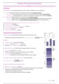
Bar Chart →
• Vertical or horizontal bars for each category.
• Frequency is shown as height/length of the bar.
• Bars have equal width & equal gap between them.
Segmented Bar Chart → bar chart with each category stacked in one column.
• Frequency shown on the vertical axis.
• Height of each segment represents the frequency of each category.
• Total length of the bar represents the total frequency.
• Give a key to the graph to show which segment represents which category.
Percentage Frequency Segmented Bar Chart → always equal 100%
frequency
Percentage frequency = × 100
total frequency
Describing the Distribution of Categorical Data:
• The mode is the only measure of centre.
• An interpretation of frequency tables, bar charts & segmented bar charts in a report should:
- Summarise the data type and the number of values in the data set
- Identify the modal category (if obvious)
- Compare the percentage frequencies of different categories
P a g e 1 | 20
, General Maths Bound Reference
Displaying Numerical Data
Dot Plots → display discrete numerical data using one for each data point on single axis.
• Small to medium sized data sets with a small range of values.
• Spacing between the dots should be consistent so the frequencies can be compared.
• Positive Skew → Tail to the Right
• Negative Skew → Tail to the Left
Stem & Leaf Plots → represent numerical data separated into:
• The leftmost digit (the stem)
• The remaining digits (the leaves)
• Small/medium sized data sets with a large range of values.
Grouped Frequency Tables → group continuous numerical data in regular intervals, displaying
distribution of data.
• Lower bound is inclusive, the upper bound is not.
• Discrete data can also be grouped when variable can take a large range of values.
Histograms → graphical displays of grouped frequency tables & numerical data.
• Provides info about the centre, spread, shape, and outlier(s) of the distribution.
• A histogram is constructed in the following way:
- Frequency (or relative frequency) → vertical axis.
- Value → horizontal axis (ungrouped discrete value → middle of column).
- There are no gaps between columns.
Log Scales →
• If 𝑥𝑥 = 1, then log(𝑥𝑥) is zero. CAS Method:
• If 0 < 𝑥𝑥 < 1, then log(𝑥𝑥) is negative.
1. 𝐶𝐶𝐶𝐶𝐶𝐶𝐶𝐶 + 10𝑥𝑥
• If 𝑥𝑥 ≤ 0, then log(𝑥𝑥) is undefined.
2. log10 𝑥𝑥
Log (0.1) = -1 Log (0.01) = -2 Log (0.001) = -3 Log (3017) = 3.48
Log (1) = 0 Log (10) = 1 Log (100) = 2 Log (1207820) = 6.08
Log (104 ) = 4 Log (106 ) = 6 Log (10−5 ) = -5 Log (62) = 1.79
CAS Method:
Displaying with Logarithmic Scale →
• Large range of data 1. Calculate the appropriate log value
• Non-linear scale that does not ↑by + equally sizes units, instead × by 2. log10 10 = 1
consistent scale factor 3. on the scale, 10 is plotted at 1
Exercise Example:
1. Calculate the appropriate log value
2. log10 1 = 0
3. This means on the log scale, 1 is plotted as 0
Five Figure Summary & Box Plots
• Minimum → smallest value
• Q1 Lower Quartile → value at 25%
• Median → value at 50%
• Q3 Upper Quartile → value at 75%
• Maximum → largest value
, General Maths Bound Reference
Finding the Range (measure of the spread) → Maximum − Minimum
Finding the Median:
• Make sure the values are in order.
• Find the value in the middle
n+1
• � th value� → n = the total number of values
2
Interquartile Range (IQR) → difference between the quartiles (IQR = Q3 – Q1).
• Measures spread of data around the median → spread of the middle 50% of the data values.
- Q1 – the first or lower quartile (median of the lower half of values)
- Q3 – third or upper quartile (median of the upper half of values)
• The IQR is not influenced by extreme values (outliers)
• Number of values (n) is odd → median (Q2) is not included in the calculation of the 1st or 3rd quartile.
• The IQR is a more useful measure of spread than the range.
Boxplots → graphical representations of the five-figure summary.
Outliers are an extreme value at one end of the data.
• Lower fence = Q1 – (1.5 x IQR)
• Upper fence = Q3 + (1.5 x IQR)
Note:
- It is not necessary to draw fences on boxplot
- The whiskers move into the first value that is not an outlier.
Exercise Example: Construct a five-number summary for the following data
3 5 1 10 8 9 6 3 8 6
Minimum – 1, Q1 – 3, Median – 6, Q3 – 8, Maximum – 10
Describing Numerical Data
Shape →
Positively Skewed → distribution trails Negatively Skewed → distribution trails Outliers → use median as centre
off in a positive (right) direction on off in a negative (left) direction on
horizontal axis. Use median as centre horizontal axis. Use median as centre
Symmetric Distribution → distribution is same on both sides of Centre → the middle of the distribution. Either
centre. Not exactly symmetric → Approx Symmetric. Use mean as mean or median can be used
centre
Same shape,
different centres →
Chapter 1
Types of Data
Univariate Data → one variable (eg. height, eye colour, number of siblings, score on a maths test)
• Numerical (discrete/continuous) → quantitative data that can be counted or measured
- Discrete → numerical data that only consists of a set of fixed values within a range (eg. whole numbers)
- Continuous → numerical data that can consist of any value within a range (eg. whole numbers & decimals)
• Categorical → qualitative data that can be organised into categories or groups
- Nominal → categorical data that cannot be sorted into a logical ordered list or hierarchy (eg. type of bread)
- Ordinal → categorical data that can be ordered into a logical ordered list or hierarchy (eg. drink size)
Exercise Example: classify the following variables as either categorical or numerical
a) Type of pasta → Categorical
b) Number of candles → Numerical
c) Type of shoes (runners, boots, sandals, slides) → Nominal
d) Shirt size (small, medium, large) → Ordinal
e) Length (m) → Continuous
f) Number of tennis racquets → Discrete
Displaying & Describing Categorical Data
Frequency Table → table that tallies how often each value in a data set occurs.
frequency
• Recorded in frequency table as frequency or percentage frequency = × 100
total frequency
Bar Chart →
• Vertical or horizontal bars for each category.
• Frequency is shown as height/length of the bar.
• Bars have equal width & equal gap between them.
Segmented Bar Chart → bar chart with each category stacked in one column.
• Frequency shown on the vertical axis.
• Height of each segment represents the frequency of each category.
• Total length of the bar represents the total frequency.
• Give a key to the graph to show which segment represents which category.
Percentage Frequency Segmented Bar Chart → always equal 100%
frequency
Percentage frequency = × 100
total frequency
Describing the Distribution of Categorical Data:
• The mode is the only measure of centre.
• An interpretation of frequency tables, bar charts & segmented bar charts in a report should:
- Summarise the data type and the number of values in the data set
- Identify the modal category (if obvious)
- Compare the percentage frequencies of different categories
P a g e 1 | 20
, General Maths Bound Reference
Displaying Numerical Data
Dot Plots → display discrete numerical data using one for each data point on single axis.
• Small to medium sized data sets with a small range of values.
• Spacing between the dots should be consistent so the frequencies can be compared.
• Positive Skew → Tail to the Right
• Negative Skew → Tail to the Left
Stem & Leaf Plots → represent numerical data separated into:
• The leftmost digit (the stem)
• The remaining digits (the leaves)
• Small/medium sized data sets with a large range of values.
Grouped Frequency Tables → group continuous numerical data in regular intervals, displaying
distribution of data.
• Lower bound is inclusive, the upper bound is not.
• Discrete data can also be grouped when variable can take a large range of values.
Histograms → graphical displays of grouped frequency tables & numerical data.
• Provides info about the centre, spread, shape, and outlier(s) of the distribution.
• A histogram is constructed in the following way:
- Frequency (or relative frequency) → vertical axis.
- Value → horizontal axis (ungrouped discrete value → middle of column).
- There are no gaps between columns.
Log Scales →
• If 𝑥𝑥 = 1, then log(𝑥𝑥) is zero. CAS Method:
• If 0 < 𝑥𝑥 < 1, then log(𝑥𝑥) is negative.
1. 𝐶𝐶𝐶𝐶𝐶𝐶𝐶𝐶 + 10𝑥𝑥
• If 𝑥𝑥 ≤ 0, then log(𝑥𝑥) is undefined.
2. log10 𝑥𝑥
Log (0.1) = -1 Log (0.01) = -2 Log (0.001) = -3 Log (3017) = 3.48
Log (1) = 0 Log (10) = 1 Log (100) = 2 Log (1207820) = 6.08
Log (104 ) = 4 Log (106 ) = 6 Log (10−5 ) = -5 Log (62) = 1.79
CAS Method:
Displaying with Logarithmic Scale →
• Large range of data 1. Calculate the appropriate log value
• Non-linear scale that does not ↑by + equally sizes units, instead × by 2. log10 10 = 1
consistent scale factor 3. on the scale, 10 is plotted at 1
Exercise Example:
1. Calculate the appropriate log value
2. log10 1 = 0
3. This means on the log scale, 1 is plotted as 0
Five Figure Summary & Box Plots
• Minimum → smallest value
• Q1 Lower Quartile → value at 25%
• Median → value at 50%
• Q3 Upper Quartile → value at 75%
• Maximum → largest value
, General Maths Bound Reference
Finding the Range (measure of the spread) → Maximum − Minimum
Finding the Median:
• Make sure the values are in order.
• Find the value in the middle
n+1
• � th value� → n = the total number of values
2
Interquartile Range (IQR) → difference between the quartiles (IQR = Q3 – Q1).
• Measures spread of data around the median → spread of the middle 50% of the data values.
- Q1 – the first or lower quartile (median of the lower half of values)
- Q3 – third or upper quartile (median of the upper half of values)
• The IQR is not influenced by extreme values (outliers)
• Number of values (n) is odd → median (Q2) is not included in the calculation of the 1st or 3rd quartile.
• The IQR is a more useful measure of spread than the range.
Boxplots → graphical representations of the five-figure summary.
Outliers are an extreme value at one end of the data.
• Lower fence = Q1 – (1.5 x IQR)
• Upper fence = Q3 + (1.5 x IQR)
Note:
- It is not necessary to draw fences on boxplot
- The whiskers move into the first value that is not an outlier.
Exercise Example: Construct a five-number summary for the following data
3 5 1 10 8 9 6 3 8 6
Minimum – 1, Q1 – 3, Median – 6, Q3 – 8, Maximum – 10
Describing Numerical Data
Shape →
Positively Skewed → distribution trails Negatively Skewed → distribution trails Outliers → use median as centre
off in a positive (right) direction on off in a negative (left) direction on
horizontal axis. Use median as centre horizontal axis. Use median as centre
Symmetric Distribution → distribution is same on both sides of Centre → the middle of the distribution. Either
centre. Not exactly symmetric → Approx Symmetric. Use mean as mean or median can be used
centre
Same shape,
different centres →