Mathematics Teachers’ Self Study Guide
on the national Curriculum Statement
Book 2 of 2
1
, WORKING WITH GROUPED DATA
Material written by
Meg Dickson and Jackie Scheiber
RADMASTE Centre, University of the Witwatersrand
The National Curriculum Statement for Grade 10, 11 and 12 (NCS)
mentions grouped data in the following Assessment Standard in Grades 10:
10.4.1
a) Collect, organise and interpret univariate numerical data in order to
determine
• Measures of central tendency (mean, median, mode) of grouped and
ungrouped data and knows which is the most appropriate under given
conditions
• Measures of dispersion: range, percentiles, quartiles, interquartile and
semi-interquartile range
b) Represent data effectively, choosing appropriately from:
• Bar and compound bar graphs
• Histograms (grouped data)
• Frequency polygons
• Pie charts
• Line and broken line graphs
UNIVARIATE DATA
Univariate data is data concerned with a single attribute or variable.
When we graph univariate data, we do so on a pictogram, bar graph, pie
chart, histogram, frequency polygon, line or broken line graph.
Univariate data looks at the range of values, as well as the central
tendency of the values.
Examples of univariate data are:
• Height of learners in Grade 11
• Length of earthworms in a soil sample
• Number of cars manufactured in a particular year
• Number of people born in a particular year
2
,There are 2 forms of numerical data:
a) Information that is collected by counting is called discrete data. The
data is collected by counting exact amounts and you list the
information or values.
e.g. the number of children in a family; the number of children with
birthdays in January; the number of goals scored at a soccer match.
b) Continuous data values form part of a continuous scale and the
values can not all be listed,
e.g. the height of learners in a Grade 8 measured in centimetres and
fractions of a centimetre; temperature measured in degrees and
fractions of a degree.
The mass of a baby at birth is continuous data, as there is no reason
why a baby should not have a mass of 3,25167312 kg – even if there
is no scale that could measure so many decimal places. However, the
number of children born to a mother is discrete data, as decimals
make no sense when counting babies!
TABLES, LISTS AND TALLIES
When you first look at data, all you may see is a jumble of information.
You need to sort the data and record it in a way that makes more sense.
Some data is easy to sort into lists that are either numerical or
alphabetical. Other data can be sorted into tables. Some tables can be
used to keep count of the number of times a particular piece of data
occurs; such a table is called a frequency table. In a frequency table
you can also find a ‘running total’ of frequencies. This is called the
cumulative frequency. It is sometimes useful to know the running total
of the frequencies as this tells you the total number of data items at
different stages in the data set.
1) STEM AND LEAF DISPLAY
Example:
Suppose the members of your Grade 11 maths class scored the following
percentages in a maths test:
32 ; 56 ; 45 ; 78 ; 77 ; 59 ; 65 ; 54 ; 54 ; 39 ;
45 ; 44 ; 52 ; 47 ; 50 ; 52 ; 51 ; 40 ; 69 ; 72 ;
3
, 36 ; 57 ; 55 ; 47 ; 33 ; 39 ; 66 ; 61 ; 48 ; 45 ;
53 ; 57 ; 56 ; 55 ; 71 ; 63 ; 62 ; 65 ; 58 ; 55 ;
This data is discrete data. The percentages are numbers representing
the count of marks on the test scripts.
This list of numbers has little meaning as it is. However, by organising
the data into tables we can begin to make some sense out of the
numbers. One way of organising them would be in a stem & leaf plot.
3 2 3 6 9 9
4 0 4 5 5 5 7 7 8
5 0 1 2 2 3 4 4 5 5 5 6 6 7 7 8 9
6 1 2 3 5 5 6 9
7 1 2 7 8
Key: 6/2 = 62
Notice the stem and leaf display is visual representation of the data. It is
easy to see that there are more marks in the fifties than in the seventies.
2) GROUPED FREQUENCY TABLE
Another way of organising the list of marks would be to write them in a
grouped frequency table. In this sort of table the numbers are arranged
in groups or class intervals.
Maths marks:
32 ; 56 ; 45 ; 78 ; 77 ; 59 ; 65 ; 54 Rewrite the list into groups of
; 54 ; 39 ; 45 ; 44 ; 52 ; 47 ; 50 ; multiples of ten like this:
52 ; 51 ; 40 ; 69 ; 72 ; 36 ; 57 ; 55
; 47 ; 33 ; 39 ; 66 ; 61 ; 48 ; 45 ;
53 ; 57 ; 56 ; 55 ; 71 ; 63 ; 62 ; 65
marks tally frequency
30 - 39 //// 5
40 - 49
50 - 59
60 – 69
There are 5 marks in the
class interval 30 -39 70 - 79
4
on the national Curriculum Statement
Book 2 of 2
1
, WORKING WITH GROUPED DATA
Material written by
Meg Dickson and Jackie Scheiber
RADMASTE Centre, University of the Witwatersrand
The National Curriculum Statement for Grade 10, 11 and 12 (NCS)
mentions grouped data in the following Assessment Standard in Grades 10:
10.4.1
a) Collect, organise and interpret univariate numerical data in order to
determine
• Measures of central tendency (mean, median, mode) of grouped and
ungrouped data and knows which is the most appropriate under given
conditions
• Measures of dispersion: range, percentiles, quartiles, interquartile and
semi-interquartile range
b) Represent data effectively, choosing appropriately from:
• Bar and compound bar graphs
• Histograms (grouped data)
• Frequency polygons
• Pie charts
• Line and broken line graphs
UNIVARIATE DATA
Univariate data is data concerned with a single attribute or variable.
When we graph univariate data, we do so on a pictogram, bar graph, pie
chart, histogram, frequency polygon, line or broken line graph.
Univariate data looks at the range of values, as well as the central
tendency of the values.
Examples of univariate data are:
• Height of learners in Grade 11
• Length of earthworms in a soil sample
• Number of cars manufactured in a particular year
• Number of people born in a particular year
2
,There are 2 forms of numerical data:
a) Information that is collected by counting is called discrete data. The
data is collected by counting exact amounts and you list the
information or values.
e.g. the number of children in a family; the number of children with
birthdays in January; the number of goals scored at a soccer match.
b) Continuous data values form part of a continuous scale and the
values can not all be listed,
e.g. the height of learners in a Grade 8 measured in centimetres and
fractions of a centimetre; temperature measured in degrees and
fractions of a degree.
The mass of a baby at birth is continuous data, as there is no reason
why a baby should not have a mass of 3,25167312 kg – even if there
is no scale that could measure so many decimal places. However, the
number of children born to a mother is discrete data, as decimals
make no sense when counting babies!
TABLES, LISTS AND TALLIES
When you first look at data, all you may see is a jumble of information.
You need to sort the data and record it in a way that makes more sense.
Some data is easy to sort into lists that are either numerical or
alphabetical. Other data can be sorted into tables. Some tables can be
used to keep count of the number of times a particular piece of data
occurs; such a table is called a frequency table. In a frequency table
you can also find a ‘running total’ of frequencies. This is called the
cumulative frequency. It is sometimes useful to know the running total
of the frequencies as this tells you the total number of data items at
different stages in the data set.
1) STEM AND LEAF DISPLAY
Example:
Suppose the members of your Grade 11 maths class scored the following
percentages in a maths test:
32 ; 56 ; 45 ; 78 ; 77 ; 59 ; 65 ; 54 ; 54 ; 39 ;
45 ; 44 ; 52 ; 47 ; 50 ; 52 ; 51 ; 40 ; 69 ; 72 ;
3
, 36 ; 57 ; 55 ; 47 ; 33 ; 39 ; 66 ; 61 ; 48 ; 45 ;
53 ; 57 ; 56 ; 55 ; 71 ; 63 ; 62 ; 65 ; 58 ; 55 ;
This data is discrete data. The percentages are numbers representing
the count of marks on the test scripts.
This list of numbers has little meaning as it is. However, by organising
the data into tables we can begin to make some sense out of the
numbers. One way of organising them would be in a stem & leaf plot.
3 2 3 6 9 9
4 0 4 5 5 5 7 7 8
5 0 1 2 2 3 4 4 5 5 5 6 6 7 7 8 9
6 1 2 3 5 5 6 9
7 1 2 7 8
Key: 6/2 = 62
Notice the stem and leaf display is visual representation of the data. It is
easy to see that there are more marks in the fifties than in the seventies.
2) GROUPED FREQUENCY TABLE
Another way of organising the list of marks would be to write them in a
grouped frequency table. In this sort of table the numbers are arranged
in groups or class intervals.
Maths marks:
32 ; 56 ; 45 ; 78 ; 77 ; 59 ; 65 ; 54 Rewrite the list into groups of
; 54 ; 39 ; 45 ; 44 ; 52 ; 47 ; 50 ; multiples of ten like this:
52 ; 51 ; 40 ; 69 ; 72 ; 36 ; 57 ; 55
; 47 ; 33 ; 39 ; 66 ; 61 ; 48 ; 45 ;
53 ; 57 ; 56 ; 55 ; 71 ; 63 ; 62 ; 65
marks tally frequency
30 - 39 //// 5
40 - 49
50 - 59
60 – 69
There are 5 marks in the
class interval 30 -39 70 - 79
4