Lecture 1 Review
● Ordinal cannot be shuffled in such a way that makes sense
● When make a claim make it about the parameter (population)
● Mu is unknown unless took a census (rare)
● Associated = dependent = paired samples (ex/ twins)
○ Have to be same size
● No association = independent = not paired samples
○ Not the same size
Lecture 2 Comparing Two Means from Independent Samples
● Parameter = mu1 - mu2 (difference between independent samples)
● Point estimate = x1 - x2 = mu1 - mu2
● As sample size increases variance decreases
● The calculation of the variance is by addition
○ More variability/error when have two things
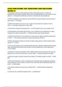
● Standard error = standard deviation
● For sd first sum then square root
● 95%(CL) of intervals contain this value
● T Test: do not know sd or sample size not big enough (need df)
○ As long as one sample size is small have to use t-test
● For DF: use the smallest # between n1 - 1 and n2 -1
● Two-sample t-test: to compare the difference in means (independent)
● Paired t-test: compare two samples from same population same variable two different
times (dependent)
Lecture 3: Comparing Two Means from Independent Samples (Cont’t)
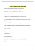
● T star = (p = 1 - alpha/2, df, lower.tail)
● If 0 is not in the confidence interval then there is a significant difference
if know the variances, otherwise use above
● Type one error = lower alpha Type two error = increase alpha
● Things that happen by chance are between -1.9 to 1.9 (for test_stat)
, Square root of the sums 1
Lecture 4: Comparing Two Proportions
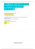
● Need 10 successes and 10 failures or else data = skewed and CLT does not apply
sum, then square root (SE for CI)
= Confidence Interval
● Change percentage to decimals
● Narrow CI raise alpha
SE for null hypothesis/HT
Lecture 5: ANOVA
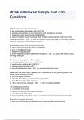
● F-statistic should equal about one
○ If the top number is larger than leans towards rejecting the null
Lecture 5: ANOVA (cont’d from understanding the ANOVA table)
● X with two bars is the grand mean (the mean of all means)
● In the df calculation no longer have k factors have k -1 because one of them gets lost in
the process b/c the third # is bound to the mean (?)
● Reasonably symmetric, no outliers at most 1 - conditions for ANOVA for R assignment
Lecture 6:ANOVA (cont’d from Back to the Example)
● In one way anova test - statistics
○ as a measure of variation among the sample means - MSTR
○ (b) as a measure of variation within the samples - MSE
● Ordinal cannot be shuffled in such a way that makes sense
● When make a claim make it about the parameter (population)
● Mu is unknown unless took a census (rare)
● Associated = dependent = paired samples (ex/ twins)
○ Have to be same size
● No association = independent = not paired samples
○ Not the same size
Lecture 2 Comparing Two Means from Independent Samples
● Parameter = mu1 - mu2 (difference between independent samples)
● Point estimate = x1 - x2 = mu1 - mu2
● As sample size increases variance decreases
● The calculation of the variance is by addition
○ More variability/error when have two things
● Standard error = standard deviation
● For sd first sum then square root
● 95%(CL) of intervals contain this value
● T Test: do not know sd or sample size not big enough (need df)
○ As long as one sample size is small have to use t-test
● For DF: use the smallest # between n1 - 1 and n2 -1
● Two-sample t-test: to compare the difference in means (independent)
● Paired t-test: compare two samples from same population same variable two different
times (dependent)
Lecture 3: Comparing Two Means from Independent Samples (Cont’t)
● T star = (p = 1 - alpha/2, df, lower.tail)
● If 0 is not in the confidence interval then there is a significant difference
if know the variances, otherwise use above
● Type one error = lower alpha Type two error = increase alpha
● Things that happen by chance are between -1.9 to 1.9 (for test_stat)
, Square root of the sums 1
Lecture 4: Comparing Two Proportions
● Need 10 successes and 10 failures or else data = skewed and CLT does not apply
sum, then square root (SE for CI)
= Confidence Interval
● Change percentage to decimals
● Narrow CI raise alpha
SE for null hypothesis/HT
Lecture 5: ANOVA
● F-statistic should equal about one
○ If the top number is larger than leans towards rejecting the null
Lecture 5: ANOVA (cont’d from understanding the ANOVA table)
● X with two bars is the grand mean (the mean of all means)
● In the df calculation no longer have k factors have k -1 because one of them gets lost in
the process b/c the third # is bound to the mean (?)
● Reasonably symmetric, no outliers at most 1 - conditions for ANOVA for R assignment
Lecture 6:ANOVA (cont’d from Back to the Example)
● In one way anova test - statistics
○ as a measure of variation among the sample means - MSTR
○ (b) as a measure of variation within the samples - MSE