https://www.stuvia.com/en-us/doc/8364376/solutions-manual-for-stochastic-processes-with-r-an-introduction-1st-
edition-by-korosteleva-2024-all-9-chapters-covered
ALL 9 CHAPTER COVERED
SOLUTIONS MANUAL
, TABLE OF CONTENTS
CHAPTER 1 ……………………………………………………………………………………. 3
CHAPTER 2 ……………………………………………………………………………………. 31
CHAPTER 3 ……………………………………………………………………………………. 41
CHAPTER 4 ……………………………………………………………………………………. 48
CHAPTER 5 ……………………………………………………………………………………. 60
CHAPTER 6 ……………………………………………………………………………………. 67
CHAPTER 7 ……………………………………………………………………………………. 74
CHAPTER 8 ……………………………………………………………………………………. 81
CHAPTER 9 ……………………………………………………………………………………. 87
2
, CHAPTER 1
0.3 0.4 0.3
EXERCISE 1.1. For a Markov chain with a one-step transition probability matrix � 0.2 0.3 0.5 �
0.8 0.1 0.1
we compute:
(a) 𝑃𝑃(𝑋𝑋3 = 2 |𝑋𝑋0 = 1, 𝑋𝑋1 = 2, 𝑋𝑋2 = 3) = 𝑃𝑃(𝑋𝑋3 = 2 | 𝑋𝑋2 = 3) (by the Markov property)
= 𝑃𝑃32 = 0.1.
(b) 𝑃𝑃(𝑋𝑋4 = 3 |𝑋𝑋0 = 2, 𝑋𝑋3 = 1) = 𝑃𝑃(𝑋𝑋4 = 3 | 𝑋𝑋3 = 1) (by the Markov property)
= 𝑃𝑃13 = 0.3.
(c) 𝑃𝑃(𝑋𝑋0 = 1, 𝑋𝑋1 = 2, 𝑋𝑋2 = 3, 𝑋𝑋3 = 1) = 𝑃𝑃(𝑋𝑋3 = 1 | 𝑋𝑋0 = 1, 𝑋𝑋1 = 2, 𝑋𝑋2 = 3) 𝑃𝑃(𝑋𝑋2 = 3 |𝑋𝑋0 = 1,
𝑋𝑋1 = 2) 𝑃𝑃(𝑋𝑋1 = 2 | 𝑋𝑋0 = 1) 𝑃𝑃(𝑋𝑋0 = 1) (by conditioning)
= 𝑃𝑃(𝑋𝑋3 = 1 | 𝑋𝑋2 = 3) 𝑃𝑃(𝑋𝑋2 = 3 | 𝑋𝑋1 = 2) 𝑃𝑃(𝑋𝑋1 = 2 | 𝑋𝑋0 = 1) 𝑃𝑃(𝑋𝑋0 = 1) (by the Markov property)
= 𝑃𝑃31 𝑃𝑃23 𝑃𝑃12 𝑃𝑃(𝑋𝑋0 = 1) = (0.8)(0.5)(0.4)(1) = 0.16.
(d) We first compute the two-step transition probability matrix. We obtain
0.3 0.4 0.3 0.3 0.4 0.3 0.41 0.27 0.32
𝐏𝐏(2) = � 0.2 0.3 0.5 � � 0.2 0.3 0.5 � = � 0.52 0.22 0.26�.
Now we write 0.8 0.1 0.1 0.8 0.1 0.1 0.34 0.36 0.30
𝑃𝑃(𝑋𝑋0 = 1, 𝑋𝑋1 = 2, 𝑋𝑋3 = 3, 𝑋𝑋5 = 1) = 𝑃𝑃(𝑋𝑋5 = 1 | 𝑋𝑋0 = 1, 𝑋𝑋1 = 2, 𝑋𝑋3 = 3) 𝑃𝑃(𝑋𝑋3 = 3 |𝑋𝑋0 = 1,
𝑋𝑋1 = 2) 𝑃𝑃(𝑋𝑋1 = 2 | 𝑋𝑋0 = 1) 𝑃𝑃(𝑋𝑋0 = 1) (by conditioning)
= 𝑃𝑃(𝑋𝑋5 = 1 | 𝑋𝑋3 = 3) 𝑃𝑃(𝑋𝑋3 = 3 | 𝑋𝑋1 = 2) 𝑃𝑃(𝑋𝑋1 = 2 | 𝑋𝑋0 = 1) 𝑃𝑃(𝑋𝑋0 = 1) (by the Markov property)
(2) (2) 𝑃𝑃(𝑋𝑋 = 1) = (0.34)(0.26)(0.4)(1) = 0.03536.
𝑃𝑃
= 𝑃𝑃31 𝑃𝑃23 12 0
EXERCISE 1.2. (a) We plot a diagram of the Markov chain.
#specifying transition probability matrix
tm<- matrix(c(1, 0, 0, 0, 0, 0.5, 0, 0, 0, 0.5, 0.2, 0, 0, 0, 0.8,
0, 0, 1, 0, 0, 0, 0, 0, 1, 0), nrow=5, ncol=5, byrow=TRUE)
#transposing transition probability matrix
tm.tr<- t(tm)
#plotting diagram
library(diagram)
plotmat(tm.tr, arr.length=0.25, arr.width=0.1, box.col="light blue",
box.lwd=1, box.prop=0.5, box.size=0.12, box.type="circle", cex.txt=0.8,
lwd=1, self.cex=0.3, self.shiftx=0.01, self.shifty=0.09)
3
, State 2 is reflective. The chain leaves that state in one step. Therefore, it forms a separate transient
class that has an infinite period.
Finally, states 3, 4, and 5 communicate and thus belong to the same class. The chain can return to
either state in this class in 3, 6, 9, etc. steps, thus the period is equal to 3. Since there is a positive
probability to leave this class, it is transient.
The R output supports these findings.
#creating Markov chain object
library(markovchain)
mc<- new("markovchain", transitionMatrix=tm,states=c("1", "2", "3", "4", "5"))
#computing Markov chain characteristics
recurrentClasses(mc)
"1"
transientClasses(mc)
"2"
"3" "4" "5"
absorbingStates(mc)
"1"
(c) Below we simulate three trajectories of the chain that start at a randomly chosen state.
4
edition-by-korosteleva-2024-all-9-chapters-covered
ALL 9 CHAPTER COVERED
SOLUTIONS MANUAL
, TABLE OF CONTENTS
CHAPTER 1 ……………………………………………………………………………………. 3
CHAPTER 2 ……………………………………………………………………………………. 31
CHAPTER 3 ……………………………………………………………………………………. 41
CHAPTER 4 ……………………………………………………………………………………. 48
CHAPTER 5 ……………………………………………………………………………………. 60
CHAPTER 6 ……………………………………………………………………………………. 67
CHAPTER 7 ……………………………………………………………………………………. 74
CHAPTER 8 ……………………………………………………………………………………. 81
CHAPTER 9 ……………………………………………………………………………………. 87
2
, CHAPTER 1
0.3 0.4 0.3
EXERCISE 1.1. For a Markov chain with a one-step transition probability matrix � 0.2 0.3 0.5 �
0.8 0.1 0.1
we compute:
(a) 𝑃𝑃(𝑋𝑋3 = 2 |𝑋𝑋0 = 1, 𝑋𝑋1 = 2, 𝑋𝑋2 = 3) = 𝑃𝑃(𝑋𝑋3 = 2 | 𝑋𝑋2 = 3) (by the Markov property)
= 𝑃𝑃32 = 0.1.
(b) 𝑃𝑃(𝑋𝑋4 = 3 |𝑋𝑋0 = 2, 𝑋𝑋3 = 1) = 𝑃𝑃(𝑋𝑋4 = 3 | 𝑋𝑋3 = 1) (by the Markov property)
= 𝑃𝑃13 = 0.3.
(c) 𝑃𝑃(𝑋𝑋0 = 1, 𝑋𝑋1 = 2, 𝑋𝑋2 = 3, 𝑋𝑋3 = 1) = 𝑃𝑃(𝑋𝑋3 = 1 | 𝑋𝑋0 = 1, 𝑋𝑋1 = 2, 𝑋𝑋2 = 3) 𝑃𝑃(𝑋𝑋2 = 3 |𝑋𝑋0 = 1,
𝑋𝑋1 = 2) 𝑃𝑃(𝑋𝑋1 = 2 | 𝑋𝑋0 = 1) 𝑃𝑃(𝑋𝑋0 = 1) (by conditioning)
= 𝑃𝑃(𝑋𝑋3 = 1 | 𝑋𝑋2 = 3) 𝑃𝑃(𝑋𝑋2 = 3 | 𝑋𝑋1 = 2) 𝑃𝑃(𝑋𝑋1 = 2 | 𝑋𝑋0 = 1) 𝑃𝑃(𝑋𝑋0 = 1) (by the Markov property)
= 𝑃𝑃31 𝑃𝑃23 𝑃𝑃12 𝑃𝑃(𝑋𝑋0 = 1) = (0.8)(0.5)(0.4)(1) = 0.16.
(d) We first compute the two-step transition probability matrix. We obtain
0.3 0.4 0.3 0.3 0.4 0.3 0.41 0.27 0.32
𝐏𝐏(2) = � 0.2 0.3 0.5 � � 0.2 0.3 0.5 � = � 0.52 0.22 0.26�.
Now we write 0.8 0.1 0.1 0.8 0.1 0.1 0.34 0.36 0.30
𝑃𝑃(𝑋𝑋0 = 1, 𝑋𝑋1 = 2, 𝑋𝑋3 = 3, 𝑋𝑋5 = 1) = 𝑃𝑃(𝑋𝑋5 = 1 | 𝑋𝑋0 = 1, 𝑋𝑋1 = 2, 𝑋𝑋3 = 3) 𝑃𝑃(𝑋𝑋3 = 3 |𝑋𝑋0 = 1,
𝑋𝑋1 = 2) 𝑃𝑃(𝑋𝑋1 = 2 | 𝑋𝑋0 = 1) 𝑃𝑃(𝑋𝑋0 = 1) (by conditioning)
= 𝑃𝑃(𝑋𝑋5 = 1 | 𝑋𝑋3 = 3) 𝑃𝑃(𝑋𝑋3 = 3 | 𝑋𝑋1 = 2) 𝑃𝑃(𝑋𝑋1 = 2 | 𝑋𝑋0 = 1) 𝑃𝑃(𝑋𝑋0 = 1) (by the Markov property)
(2) (2) 𝑃𝑃(𝑋𝑋 = 1) = (0.34)(0.26)(0.4)(1) = 0.03536.
𝑃𝑃
= 𝑃𝑃31 𝑃𝑃23 12 0
EXERCISE 1.2. (a) We plot a diagram of the Markov chain.
#specifying transition probability matrix
tm<- matrix(c(1, 0, 0, 0, 0, 0.5, 0, 0, 0, 0.5, 0.2, 0, 0, 0, 0.8,
0, 0, 1, 0, 0, 0, 0, 0, 1, 0), nrow=5, ncol=5, byrow=TRUE)
#transposing transition probability matrix
tm.tr<- t(tm)
#plotting diagram
library(diagram)
plotmat(tm.tr, arr.length=0.25, arr.width=0.1, box.col="light blue",
box.lwd=1, box.prop=0.5, box.size=0.12, box.type="circle", cex.txt=0.8,
lwd=1, self.cex=0.3, self.shiftx=0.01, self.shifty=0.09)
3
, State 2 is reflective. The chain leaves that state in one step. Therefore, it forms a separate transient
class that has an infinite period.
Finally, states 3, 4, and 5 communicate and thus belong to the same class. The chain can return to
either state in this class in 3, 6, 9, etc. steps, thus the period is equal to 3. Since there is a positive
probability to leave this class, it is transient.
The R output supports these findings.
#creating Markov chain object
library(markovchain)
mc<- new("markovchain", transitionMatrix=tm,states=c("1", "2", "3", "4", "5"))
#computing Markov chain characteristics
recurrentClasses(mc)
"1"
transientClasses(mc)
"2"
"3" "4" "5"
absorbingStates(mc)
"1"
(c) Below we simulate three trajectories of the chain that start at a randomly chosen state.
4