The Market System – Lecture 3
1. The perfect market assumption
1.1. Perfect market assumption
• The perfect market assumptions:
➢ Perfect knowledge : Households have information on the qualities and prices of everything available in
the market, and firms have all available information on wage rates, capital costs, technology, and output
prices
➢ Perfect competition : Many small buyers and sellers → no individual can influence market prices
➢ Homogeneous products : Goods are identical, no differentiation
BUT: not for everyone: eg coca cola & pepsi
2. Household budget constraint
2.1. Household behavior and consumer choice
• Every day people make various decisions
➢ Output market decisions: what to buy & how much to buy
➢ Input market decisions: how much labor to supply, to spend now & save for the future
• Choices are constrained (beperkt) → Households make constrained choices
➢ Income → limits consumption
➢ Time → limits labor suppl
2.2. The budget constraint
• The household faces a budget constraint
➢ A household’s spending choices are limited by its income, wealth, expectations (about income & wealth)
& product prices
• The household has a choice set / opportunity set
➢ The set of options that is defined & limited by a budget constraint
2.3. Opportunity costs
• Preferences & tastes
➢ Households choose freely within their budget limits, guided by personal preferences
• Trade-offs
➢ Every purchase (aankoop) involves comparing the chosen product to all other alternatives that could be
bought with the same money
• Opportunity cost
➢ With a limited budget, the real cost of any product is the value of the other goods and services that could
have been purchased with the same amount of money
2.4. The budget constraint
• Budget constraint
➢ Defines which product combinations a household can afford
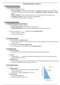
with its limited income
➔ Points A, C, and D are affordable; Point E is not
• Opportunity set
➢ The available combinations
➢ Influenced by both prices & income
, • General the budget = 𝑷𝑿𝑿+𝑷𝒀𝒀=I
➢ PX , PY = price of X & Y
➢ X , Y = quantity of X & Y consumed
➢ I = household income
• Effects on the Budged line
➢ Price change
Price of a good ↓ → budget line rotates outward (right)
→ increased available opportunities and an expanded choice set
Price of a good ↑ → budget line rotates inward (left)
→ reduced available opportunities and a reduced choice set
➢ Budget shift
Income ↓ → budget line shifts left
→ decreased available opportunities and a reduced choice set
Income ↑ → budget line shifts right
→ increased available opportunities and an expanded choice set
2.5. Nominal versus real income
• Nominal income
➢ Income measured in terms of money (without adjustment for inflation)
• Real income
➢ the purchasing power of a household’s nominal income, adjusted for changes in price levels
𝒏𝒐𝒎𝒊𝒏𝒂𝒍 𝒊𝒏𝒄𝒐𝒎𝒆
➢ Income adjusted for inflation: real income =
𝒑𝒓𝒊𝒄𝒆 𝒍𝒆𝒗𝒆𝒍
➢ Real income ↑ when nominal income ↑ or/and when prices ↓
➢ Real income ↓ when nominal income ↓ or/and when prices ↑
3. Utility as the basis of household choice
• Utility: satisfaction from consumptiom of a product
• Marginal utility : extra satisfaction from one more unit
• Total utility: total satisfaction
• Law of diminishing marginal utility
➢ As consumption increases, the marginal utility decreases
Remark: opposite products: sports, drugs …
4. Indifference curves
• Indifference curve: combinations of goods X and Y that have equal utility
• Preference map: set of indifference curves
➢ Higher indifference curves = higher levels of utility
• Slope of the indifference curve is negative and decreases in
absolute value with X
• Slope of the indifference curve:
➢ 𝑀𝑈𝑋 ∆𝑋 =−(𝑀𝑈𝑌 ∆𝑌)
∆Y MUX
=-
∆X MUY
➢ 𝑀𝑈𝑋 = marginal utility derived from consuming an additional
unit (or the last unit) of X
➢ 𝑀𝑈𝑌 = marginal utility derived from consuming an additional
unit (or the last unit) of Y
1. The perfect market assumption
1.1. Perfect market assumption
• The perfect market assumptions:
➢ Perfect knowledge : Households have information on the qualities and prices of everything available in
the market, and firms have all available information on wage rates, capital costs, technology, and output
prices
➢ Perfect competition : Many small buyers and sellers → no individual can influence market prices
➢ Homogeneous products : Goods are identical, no differentiation
BUT: not for everyone: eg coca cola & pepsi
2. Household budget constraint
2.1. Household behavior and consumer choice
• Every day people make various decisions
➢ Output market decisions: what to buy & how much to buy
➢ Input market decisions: how much labor to supply, to spend now & save for the future
• Choices are constrained (beperkt) → Households make constrained choices
➢ Income → limits consumption
➢ Time → limits labor suppl
2.2. The budget constraint
• The household faces a budget constraint
➢ A household’s spending choices are limited by its income, wealth, expectations (about income & wealth)
& product prices
• The household has a choice set / opportunity set
➢ The set of options that is defined & limited by a budget constraint
2.3. Opportunity costs
• Preferences & tastes
➢ Households choose freely within their budget limits, guided by personal preferences
• Trade-offs
➢ Every purchase (aankoop) involves comparing the chosen product to all other alternatives that could be
bought with the same money
• Opportunity cost
➢ With a limited budget, the real cost of any product is the value of the other goods and services that could
have been purchased with the same amount of money
2.4. The budget constraint
• Budget constraint
➢ Defines which product combinations a household can afford
with its limited income
➔ Points A, C, and D are affordable; Point E is not
• Opportunity set
➢ The available combinations
➢ Influenced by both prices & income
, • General the budget = 𝑷𝑿𝑿+𝑷𝒀𝒀=I
➢ PX , PY = price of X & Y
➢ X , Y = quantity of X & Y consumed
➢ I = household income
• Effects on the Budged line
➢ Price change
Price of a good ↓ → budget line rotates outward (right)
→ increased available opportunities and an expanded choice set
Price of a good ↑ → budget line rotates inward (left)
→ reduced available opportunities and a reduced choice set
➢ Budget shift
Income ↓ → budget line shifts left
→ decreased available opportunities and a reduced choice set
Income ↑ → budget line shifts right
→ increased available opportunities and an expanded choice set
2.5. Nominal versus real income
• Nominal income
➢ Income measured in terms of money (without adjustment for inflation)
• Real income
➢ the purchasing power of a household’s nominal income, adjusted for changes in price levels
𝒏𝒐𝒎𝒊𝒏𝒂𝒍 𝒊𝒏𝒄𝒐𝒎𝒆
➢ Income adjusted for inflation: real income =
𝒑𝒓𝒊𝒄𝒆 𝒍𝒆𝒗𝒆𝒍
➢ Real income ↑ when nominal income ↑ or/and when prices ↓
➢ Real income ↓ when nominal income ↓ or/and when prices ↑
3. Utility as the basis of household choice
• Utility: satisfaction from consumptiom of a product
• Marginal utility : extra satisfaction from one more unit
• Total utility: total satisfaction
• Law of diminishing marginal utility
➢ As consumption increases, the marginal utility decreases
Remark: opposite products: sports, drugs …
4. Indifference curves
• Indifference curve: combinations of goods X and Y that have equal utility
• Preference map: set of indifference curves
➢ Higher indifference curves = higher levels of utility
• Slope of the indifference curve is negative and decreases in
absolute value with X
• Slope of the indifference curve:
➢ 𝑀𝑈𝑋 ∆𝑋 =−(𝑀𝑈𝑌 ∆𝑌)
∆Y MUX
=-
∆X MUY
➢ 𝑀𝑈𝑋 = marginal utility derived from consuming an additional
unit (or the last unit) of X
➢ 𝑀𝑈𝑌 = marginal utility derived from consuming an additional
unit (or the last unit) of Y