Summary Master Microsoft Excel: Formatting and Data Validation

Excel conditional formatting and data validation:

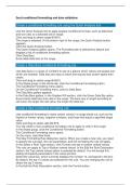
Create a conditional formatting rule using the Quick Analysis tool

Use the Quick Analysis tool to apply popular conditional formats, such as data bars
and icon sets, to a selected cell or range.
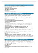
Click and drag to select range B4:B15.
The range is selected. At the bottom-right of the range, the Quick Analysis button
appears.
Click the Quick Analysis button.
The Quick Analysis gallery opens. The Formatting tab is selected by default and
displays a list of conditional formatting options.
Click Data Bars.
Excel adds data bars to the range.

Create a Data Bars conditional formatting rule

Use data bars in a range of numbers to see at a glance which values are largest and
which are smallest. Data bars are easy to insert and require less screen space than
charts.
Click and drag to select range B4:B15.
In the Styles group on the Home tab, click the Conditional Formatting button.
The Conditional Formatting menu opens.
On the Conditional Formatting menu, point to Data Bars.
The Data Bars gallery appears.
In the Data Bars gallery, in the Gradient Fill section, click the Green Data Bar option.
Excel inserts data bars into cells in the range. The bars vary in length according to
cell value; the larger the cell value, the longer the data bar.

Create a New conditional formatting rule

Use conditional formatting to make certain values in a range stand out, such as the
highest or lowest values, negative numbers, and those that equal a specified target
value.
Click and drag to select cells B4:B15.
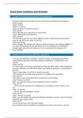
You will create a new conditional formatting rule to apply to cells in this range.
In the Styles group, click the Conditional Formatting button.
The Conditional Formatting menu opens.
On the menu, click New Rule.
The New Formatting Rule dialog box opens. When you create a new rule, you need
to specify the rule type, the rule parameters, and the formatting the rule will apply.
In the Select a Rule Type section, click Format only top or bottom ranked values.
This rule can apply to Top or Bottom ranked values. In the Edit the Rule Description
section, the Top ranked values option is selected by default. You will accept this
setting and specify parameters in the value text box.
Select the value box, which currently displays the number 10, and type 5 in the box.
By default, the top 10 values are selected for this rule. You are changing the rule to
select the top 5 values.
In the Edit the Rule Description section, click the Format button.

, The Format Cells dialog box opens, where you will choose formatting options for the
top ranked cells.
In the Format Cells dialog box, click the Fill tab.
You will fill the cell backgrounds of the top ranked cells with a color you specify here.
In the Background Color section, click the Blue, Accent 5 option, the second to last
color in the top row.
Top ranked cells will be formatted with a Blue, Accent 5 cell background.
In the Format Cells dialog box, click OK.
Excel previews the conditional formatting choice in the New Formatting Rule dialog
box.
Click OK.
Excel applies the new conditional formatting rule to the range.The top 5 cells are
highlighted in blue.

Create a Highlight Cells conditional formatting rule

Use conditional formatting rules to identify and highlight the cells in a worksheet that
contain a target value, such as test scores over 90 or the lowest unit cost.
Click and drag to select range B4:B15.
In the Styles group, click the Conditional Formatting button.
The Conditional Formatting menu opens.
On the Conditional Formatting menu, point to Highlight Cells Rules.
The Highlight Cells Rules menu opens with a variety of rule options. You can
highlight cells based on relative values, text content, dates, and more.
Click Less Than.
The Less Than dialog box opens. The insertion point is in the Format cells that are
LESS THAN text box.
Type 50000 in the text box.
Excel will highlight every cell in the selected range whose value is less than $50,000.
Next, you will choose a formatting option for highlighting the cells.
Click the Format cells arrow.
A list of formatting options appears.
On the list, click the Yellow Fill with Dark Yellow Text option.
Click OK.
Excel highlights cells in the range B4:B15 as specified in the conditional formatting
rule.

Create a Duplicate Values conditional formatting rule

Using conditional formatting to highlight duplicate values in a table can help eliminate
data entry errors or possible duplicate records. For example, you could check your
customer contact table to determine whether two companies have the same
Manager ID by mistake.
Click and drag to select range A5:J18.
In the Styles group on the Home tab, click the Conditional Formatting button.
The Conditional Formatting menu opens.
On the menu, point to Highlight Cells Rules.
The Highlight Cells Rules menu appears with a variety of options for highlighting
cells.
Click Duplicate Values.