Advanced Engineering Mathematics,
International Adaptation, 11th Edition
Erwin Kreyszig Chapter 1-25
SOLUTION MANUAL
,Table of Contents
PART A Ordinary Differential Equations (ODEs)
1. First-Order ODEs
2. Second-Order Linear ODEs
3. Higher Order Linear ODEs
4. Systems of ODEs. Phase Plane. Qualitative Methods
5. Series Solutions of ODEs. Special Functions
6. Laplace Transforms
PART B Linear Algebra. Vector Calculus
7. Linear Algebra: Matrices, Vectors, Determinants. Linear Systems
8. Linear Algebra: Matrix Eigenvalue Problems
9. Vector Differential Calculus. Grad, Div, Curl
10. Vector Integral Calculus. Integral Theorems
PART C Fourier Analysis. Partial Differential Equations (PDEs)
11. Fourier Analysis
12. Partial Differential Equations (PDEs)
PART D Complex Analysis
13. Complex Numbers and Functions. Complex Differentiation
14. Complex Integration
15. Power Series, Taylor Series
16. Laurent Series. Residue Integration
17. Conformal Mapping
PART E Numeric Analysis
18. Software
19. Numerics in General
20. Numeric Linear Algebra
21. Numerics for ODEs and PDEs
PART F Optimization, Graphs
22. Unconstrained Optimization. Linear Programming
23. Graphs: Combinatorial Optimization
24. Data Analysis: Probability Theory
25. Mathematical Statistics
, PART A
Ordinary
Differential
Equations (ODE
Chap. 1 First-Order ODEs
Sec. 1.1 Basic Concepts. Modeling
To get a good start into this chapter and this section, quickly review your basic calculus. Take a
look at the front matter of the textbook and see a review of the main differentiation and integration
formulas. Also, Appendix 3, pp. A63–A66, has useful formulas for such functions as exponential
function, logarithm, sine and cosine, etc. The beauty of ordinary differential equations is that the
subject is quite systematic and has different methods for different types of ordinary differential
equations, as you shall learn. Let us discuss some Examples of Sec. 1.1, pp. 4–7.
Example 2, p. 5. Solution by Calculus. Solution Curves. To solve the first-order
ordinary differential equation (ODE)
y′ = cos x
means that we are looking for a function whose derivative is cos x. Your first answer might be
that the desired function is sin x, because (sin x)′ = cos x. But your answer would be
incomplete because also (sin x + 2)′ = cos x, since the derivative of 2 and of any constant is
0. Hence the complete answer is y = cos x + c, where c is an arbitrary constant. As you vary
the constants you get an infinite family of solutions. Some of these solutions are shown in
Fig. 3. The lesson here is that you should never
forget your constants!
Example 4, pp. 6–7. Initial Value Problem. In an initial value problem (IVP) for a first-order
ODE we are given an ODE, here y′ = 3y, and an initial value condition y(0) = 5.7. For such a
problem, the first step is to solve the ODE. Here we obtain y(x) = ce3x as shown in Example
3, p. 5. Since we also have an initial condition, we must substitute that condition into our
solution and get y(0) = ce3·0 = ce 0 = c · 1 = c = 5.7. Hence the complete solution is y(x) = 5.7e3x
. The lesson here is that for an initial value problem you get a unique solution, also known
as a particular solution.
,2 Ordinary Differential Equations (ODEs) Part A
Modeling means that you interpret a physical problem, set up an appropriate mathematical
model, and then try to solve the mathematical formula. Finally, you have to interpret your
answer.
Examples 3 (exponential growth, exponential decay) and 5 (radioactivity) are examples of
modeling problems. Take a close look at Example 5, p. 7, because it outlines all the steps
of modeling.
Problem Set 1.1. Page 8
3. Calculus. From Example 3, replacing the independent variable t by x we know that y′ =
0.2y has a solution y = 0.2ce0.2x . Thus by analogy, y′ = y has a solution
1 · ce1·x = cex ,
where c is an arbitrary constant.
Another approach (to be discussed in details in Sec. 1.3) is to write the ODE as
dy
= y,
dx
and then by algebra
obtain 1
dy = y dx, so dy = dx.
that y
Integrate both sides, and then apply exponential functions on both sides to obtain the
same solution as above
1
dy = dx, ln |y| = x + c, eln |y| = ex+c, y = e x · e c = c ∗e x ,
y
(where c∗ = ec is a constant).
The technique used is called separation of variables because we separated the variables,
so that y
appeared on one side of the equation and x on the other side before we integrated.
7. Solve by integration. Integrating y′ = cosh 5.13x we obtain (chain rule!) y = cosh 5.13x dx
1 (sinh 5.13x) + c. Check: Differentiate your answer:
= .13
5
′
1 1
5.13 (sinh 5.13x) + = 5.13
(cosh 5.13x) · 5.13 = cosh 5.13x, which is correct.
c
11. Initial value problem (IVP). (a) Differentiation of y = (x + c)ex by product rule and definition of
y gives
y′ = ex + (x + c)ex = ex + y.
But this looks precisely like the given ODE y′ = ex + y. Hence we have shown that indeed
y = (x + c)ex is a solution of the given ODE. (b) Substitute the initial value condition into
the solution to give y(0) = (0 + c)e0 = c · 1 = 1 . Hence c = 1 so that the answer to the IVP is
2 2
y = (x + 12)ex .
(c) The graph intersects the x-axis at x = 0.5 and shoots exponentially upward.
,Chap. 1 First-Order ODEs 3
19. Modeling: Free Fall. y′′ = g = const is the model of the problem, an ODE of second order.
Integrate on both sides of the ODE with respect to t and obtain the velocity v = y′ = gt + c1
(c1 arbitrary). Integrate once more to obtain the distance fallen2 y = 1 gt2 + c1t + c2 (c2 arbitrary).
To do these steps, we used calculus. From the last equation we obtain
′ 2
y = 1 gt2 by imposing
the initial conditions y(0) = 0 and y (0) = 0, arising from the stone starting at rest at our
choice of origin, that is the initial position is y = 0 with initial velocity 0. From this we have
y(0) = c2 = 0 and v(0) = y′(0) = c1 = 0.
Sec. 1.2 Geometric Meaning of y′ = f (x, y). Direction Fields, Euler’s Method
Problem Set 1.2. Page 11
1. Direction field, verification of solution. You may verify by differentiation that the general
solution is y = tan(x + c) and the particular solution satisfying4 y( 1 π) = 1 is y = tan x. Indeed,
for the
particular solution you obtain
2 2
′ 1 sin x + cos x 2 2
y = =
cos2x = 1 + tan x = 1 + y
cos2x
and for the general solution the corresponding formula with x replaced by x + c.
y
2
y(x) 1
–1 –0.5 0 0.5 1 x
–1
–2
Sec. 1.2 Prob. 1. Direction Field
15. Initial value problem. Parachutist. In this section the usual notation is (1), that is, y′ = f
(x, y), and the direction field lies in the xy-plane. In Prob. 15 the ODE is v = f (t, v) = g −
bv2/m, where v suggests velocity. Hence the direction field lies in the tv-plane. With m = 1
and b = 1 the ODE becomes v′ = g − v2. To find the limiting velocity we find the velocity for
which the acceleration equals zero. This occurs when g − v2 = 9.80 − v2 = 0 or v = 3.13
(approximately). For v < 3.13 you have v′ > 0 (increasing curves) and for v > 3.13 you have
v′ < 0 (decreasing curves). Note that the isoclines are the horizontal parallel straight lines
g − v2 = const, thus v = const.
,4 Ordinary Differential Equations (ODEs) Part A
Sec. 1.3 Separable ODEs.
Modeling Problem Set 1.3. Page 18
1. CAUTION! Constant of integration. It is important to introduce the constant of
integration immediately, in order to avoid getting the wrong answer. For instance, let
y′ = y. Then ln |y| = x + c, y = c ∗e x (c∗ = e c),
which is the correct way to do it (the same as in Prob. 3 of Sec. 1.1 above) whereas
introducing the constant of integration later yields
y′ = y, ln |y| = x, y = ex + C
which is not a solution of y′ = y when C = 0.
5. General solution. Separating variables, we have y dy = −36x dx. By integration,
= 2c̃ − 36x2 ,
1 2 2
2y = −18x + c̃ , y = ± c − 36x2 (c = 2c̃ ).
y
2
With the plus sign of the square root we get the upper half and with the minus sign the
lower half of the ellipses in the answer on p. A4 in Appendix 2 of the textbook.
For y = 0 (the x-axis) these ellipses have a vertical tangent, so that at points of the x-axis
the derivative y′ does not exist (is infinite).
17. Initial value problem. Using the extended method (8)–(10), let u = y/x. Then by product rule
y′ = u + xu′. Now
y + 3x 4cos 2(y/x) y y
y′ = = + 3x3 cos = u + 3x3 cos2 u = u + x(3x2 cos2 u)
x x x
so that u′ = 3x2 cos2 u.
Separating variables, the last equation becomes
du 2
= 3x dx.
cos2 u
Integrate both sides, on the left with respect to u and on the right with respect to x, as justified
in the text then solve for u and express the intermediate result in terms of x and y
y
tan u = x3 + c, u= = arctan (x3 + c), y = xu = x arctan (x3 + c).
x
Substituting the initial condition into the last equation, we have
y(1) = 1 arctan (13 + c) = 0, hence c = −1.
Together we obtain the
answer
y = x arctan (x3 − 1).
23. Modeling. Boyle–Mariotte’s law for ideal gases. From the given information on the
rate of change of the volume
dV V
=− .
dP P
,Chap. 1 First-Order ODEs 5
Separating variables and integrating gives
dV 1 1
d
P
dP, ln |V | = −ln |P | + c.
P
=− , dV = −
V P V
Applying exponents to both sides and simplifying
1
eln |V | = e−ln |P|+c = e−ln |P| · ec = c c
1
·e = e .
e ln |P| |P|
Hence we obtain for nonnegative V and P the desired law (with c∗ = ec , a constant)
V · P = c∗ .
Sec. 1.4 Exact ODEs. Integrating Factors
Use (6) or (6∗), on p. 22, only if inspection fails. Use only one of the two formulas, namely, that in
which the integration is simpler. For integrating factors try both Theorems 1 and 2, on p. 25.
Usually only one of them (or sometimes neither) will work. There is no completely systematic
method for integrating factors, but these two theorems will help in many cases. Thus this section
is slightly more difficult.
Problem Set 1.4. Page 26
1. Exact ODE. We proceed as in Example 1 of Sec. 1.4. We can write the given ODE as
M dx + N dy = 0 where M = 2xy and N = x2.
∂M
Next we compute = 2x (where, when taking this partial derivative, we treat x as if it were a
∂y
∂N
constant) = 2x (we treat y as if it were a constant). (See Appendix A3.2 for a review of
and partial
∂x
derivatives.) This shows that the ODE is exact by (5) of Sec. 1.4. From (6) we obtain by
integration
u= M dx + k(y ) = 2xy dx + k(y) = x2y + k(y).
To find k(y) we differentiate this formula with respect to y and use (4b) to obtain
∂u 2 dk = N = x2.
∂ y = x + dy
From this we see
that dk
= 0, k = const.
dy
The last equation was obtained by integration. Insert this into the equation for u, compare
with (3) of Sec. 1.4, and obtain u = x2y + c∗. Because u is a constant, we have
x 2 y = c, hence y = c/x2.
,6 Ordinary Differential Equations (ODEs) Part A
5. Nonexact ODE. From the ODE, we see that P = x2 + y2 and Q = 2xy. Taking the partials we
have
∂P ∂Q
= 2y = −2y and, since they are not equal to each other, the ODE is nonexact. Trying
and ∂x
∂y
Theorem 1, p. 25, we have
(∂P/∂ y − ∂Q/∂ x ) 2y + 2y = 4y = − 2
R= =
Q −2xy −2xy x
which is a function of x only so, by (17), we have F (x) = exp R(x) dx. Now
1
R(x) dx = −2 dx = −2 ln x = ln (x−2) so that F (x) = x−2.
x
The
n ∂M ∂N
M = FP = 1 + x−2y 2 and N = FQ = −2x−1y. Thus = 2x−2y = .
∂y ∂x
This shows that multiplying by our integrating factor produced an exact ODE. We solve this
equation using 4(b), p. 21. We have
u= −2x−1y dy = −2x−1 y dy = −x−1y2 + k(x).
From this we obtain
∂u = x−2y 2 + dk dk
= M = 1 + x−2y2, so =1 and k = dx = x + c∗.
∂x that dx
d
x
Putting k into the equation for u, we obtain
u(x, y) = −x−1y2 + x + c∗ and putting it in the form of (3) u = −x−1y 2 + x = c.
Solving explicitly for y requires that we multiply both sides of the last equation by x, thereby
obtaining (with our constant = −constant on p. A5)
−y2 + x2 = cx, y = (x2 − cx)1/2.
9. Initial value problem. In this section we usually obtain an implicit rather than an explicit
general solution. The point of this problem is to illustrate that in solving initial value
problems, one can proceed directly with the implicit solution rather than first converting it to
explicit form.
The given ODE is exact because (5) gives
∂ 2x
cos y) = sin y = Nx .
My = (2e −2e2x
∂y
From this and (6) we obtain, by integration,
u= M dx = 2 e2x cos y dx = e2x cos y + k ( y).
uy = N now gives
uy = −e2x sin y + k ′ ( y) = N , k ′ ( y) = 0, k ( y) = c∗ = const.
,Chap. 1 First-Order ODEs 7
Hence an implicit general
solution is
u = e2x cos y = c.
To obtain the desired particular solution (the solution of the initial value problem), simply insert
x = 0 and y = 0 into the general solution obtained:
e0 cos 0 = 1 · 1 = c.
Hence c = 1 and the
answer is
e 2x cos y = 1.
This implies
cos y = e−2x , thus the explicit form y = arccos (e−2x ).
15. Exactness. We have M = ax + by, N = kx + ly. The answer follows from the exactness
condition (5), p. 21. The calculation is
My = b = Nx = k , M = ax + ky, u= M dx = 1 ax2 + kxy + κ( y)
2
with κ( y) to be determined from the condition
uy = kx + κ′ ( y) = N = kx + ly, hence κ′ = ly.
Integration gives κ =21 ly2. With this κ, the function u becomes
u = 1 ax2 + kxy + 1 ly2 = const.
2 2
(If we multiply the equation by a factor 2, for beauty, we obtain the answer on p. A5).
Sec. 1.5 Linear ODEs. Bernoulli Equation. Population
Dynamics Example 3, pp. 30–31. Hormone level. The
integral
πt
I= eKt cos dt
12
can be evaluated by integration by parts, as is shown in calculus, or, more simply, by
undetermined coefficients, as follows. We start from
πt πt πt
e Kt cos dt = eKt a cos + b sin
12 12 12
with a and b to be determined. Differentiation on both sides and division by eKt gives
πt π πt πt
cos =K t + b sin π t aπ b cos .
12 cos 12 − π 12
1 1 sin +
2 2 12
1
2
, 8 Ordinary Differential Equations (ODEs) Part A
THOSE WERE PREVIEW PAGES
TO DOWNLOAD THE FULL PDF
CLICK ON THE L.I.N.K
ON THE NEXT PAGE
International Adaptation, 11th Edition
Erwin Kreyszig Chapter 1-25
SOLUTION MANUAL
,Table of Contents
PART A Ordinary Differential Equations (ODEs)
1. First-Order ODEs
2. Second-Order Linear ODEs
3. Higher Order Linear ODEs
4. Systems of ODEs. Phase Plane. Qualitative Methods
5. Series Solutions of ODEs. Special Functions
6. Laplace Transforms
PART B Linear Algebra. Vector Calculus
7. Linear Algebra: Matrices, Vectors, Determinants. Linear Systems
8. Linear Algebra: Matrix Eigenvalue Problems
9. Vector Differential Calculus. Grad, Div, Curl
10. Vector Integral Calculus. Integral Theorems
PART C Fourier Analysis. Partial Differential Equations (PDEs)
11. Fourier Analysis
12. Partial Differential Equations (PDEs)
PART D Complex Analysis
13. Complex Numbers and Functions. Complex Differentiation
14. Complex Integration
15. Power Series, Taylor Series
16. Laurent Series. Residue Integration
17. Conformal Mapping
PART E Numeric Analysis
18. Software
19. Numerics in General
20. Numeric Linear Algebra
21. Numerics for ODEs and PDEs
PART F Optimization, Graphs
22. Unconstrained Optimization. Linear Programming
23. Graphs: Combinatorial Optimization
24. Data Analysis: Probability Theory
25. Mathematical Statistics
, PART A
Ordinary
Differential
Equations (ODE
Chap. 1 First-Order ODEs
Sec. 1.1 Basic Concepts. Modeling
To get a good start into this chapter and this section, quickly review your basic calculus. Take a
look at the front matter of the textbook and see a review of the main differentiation and integration
formulas. Also, Appendix 3, pp. A63–A66, has useful formulas for such functions as exponential
function, logarithm, sine and cosine, etc. The beauty of ordinary differential equations is that the
subject is quite systematic and has different methods for different types of ordinary differential
equations, as you shall learn. Let us discuss some Examples of Sec. 1.1, pp. 4–7.
Example 2, p. 5. Solution by Calculus. Solution Curves. To solve the first-order
ordinary differential equation (ODE)
y′ = cos x
means that we are looking for a function whose derivative is cos x. Your first answer might be
that the desired function is sin x, because (sin x)′ = cos x. But your answer would be
incomplete because also (sin x + 2)′ = cos x, since the derivative of 2 and of any constant is
0. Hence the complete answer is y = cos x + c, where c is an arbitrary constant. As you vary
the constants you get an infinite family of solutions. Some of these solutions are shown in
Fig. 3. The lesson here is that you should never
forget your constants!
Example 4, pp. 6–7. Initial Value Problem. In an initial value problem (IVP) for a first-order
ODE we are given an ODE, here y′ = 3y, and an initial value condition y(0) = 5.7. For such a
problem, the first step is to solve the ODE. Here we obtain y(x) = ce3x as shown in Example
3, p. 5. Since we also have an initial condition, we must substitute that condition into our
solution and get y(0) = ce3·0 = ce 0 = c · 1 = c = 5.7. Hence the complete solution is y(x) = 5.7e3x
. The lesson here is that for an initial value problem you get a unique solution, also known
as a particular solution.
,2 Ordinary Differential Equations (ODEs) Part A
Modeling means that you interpret a physical problem, set up an appropriate mathematical
model, and then try to solve the mathematical formula. Finally, you have to interpret your
answer.
Examples 3 (exponential growth, exponential decay) and 5 (radioactivity) are examples of
modeling problems. Take a close look at Example 5, p. 7, because it outlines all the steps
of modeling.
Problem Set 1.1. Page 8
3. Calculus. From Example 3, replacing the independent variable t by x we know that y′ =
0.2y has a solution y = 0.2ce0.2x . Thus by analogy, y′ = y has a solution
1 · ce1·x = cex ,
where c is an arbitrary constant.
Another approach (to be discussed in details in Sec. 1.3) is to write the ODE as
dy
= y,
dx
and then by algebra
obtain 1
dy = y dx, so dy = dx.
that y
Integrate both sides, and then apply exponential functions on both sides to obtain the
same solution as above
1
dy = dx, ln |y| = x + c, eln |y| = ex+c, y = e x · e c = c ∗e x ,
y
(where c∗ = ec is a constant).
The technique used is called separation of variables because we separated the variables,
so that y
appeared on one side of the equation and x on the other side before we integrated.
7. Solve by integration. Integrating y′ = cosh 5.13x we obtain (chain rule!) y = cosh 5.13x dx
1 (sinh 5.13x) + c. Check: Differentiate your answer:
= .13
5
′
1 1
5.13 (sinh 5.13x) + = 5.13
(cosh 5.13x) · 5.13 = cosh 5.13x, which is correct.
c
11. Initial value problem (IVP). (a) Differentiation of y = (x + c)ex by product rule and definition of
y gives
y′ = ex + (x + c)ex = ex + y.
But this looks precisely like the given ODE y′ = ex + y. Hence we have shown that indeed
y = (x + c)ex is a solution of the given ODE. (b) Substitute the initial value condition into
the solution to give y(0) = (0 + c)e0 = c · 1 = 1 . Hence c = 1 so that the answer to the IVP is
2 2
y = (x + 12)ex .
(c) The graph intersects the x-axis at x = 0.5 and shoots exponentially upward.
,Chap. 1 First-Order ODEs 3
19. Modeling: Free Fall. y′′ = g = const is the model of the problem, an ODE of second order.
Integrate on both sides of the ODE with respect to t and obtain the velocity v = y′ = gt + c1
(c1 arbitrary). Integrate once more to obtain the distance fallen2 y = 1 gt2 + c1t + c2 (c2 arbitrary).
To do these steps, we used calculus. From the last equation we obtain
′ 2
y = 1 gt2 by imposing
the initial conditions y(0) = 0 and y (0) = 0, arising from the stone starting at rest at our
choice of origin, that is the initial position is y = 0 with initial velocity 0. From this we have
y(0) = c2 = 0 and v(0) = y′(0) = c1 = 0.
Sec. 1.2 Geometric Meaning of y′ = f (x, y). Direction Fields, Euler’s Method
Problem Set 1.2. Page 11
1. Direction field, verification of solution. You may verify by differentiation that the general
solution is y = tan(x + c) and the particular solution satisfying4 y( 1 π) = 1 is y = tan x. Indeed,
for the
particular solution you obtain
2 2
′ 1 sin x + cos x 2 2
y = =
cos2x = 1 + tan x = 1 + y
cos2x
and for the general solution the corresponding formula with x replaced by x + c.
y
2
y(x) 1
–1 –0.5 0 0.5 1 x
–1
–2
Sec. 1.2 Prob. 1. Direction Field
15. Initial value problem. Parachutist. In this section the usual notation is (1), that is, y′ = f
(x, y), and the direction field lies in the xy-plane. In Prob. 15 the ODE is v = f (t, v) = g −
bv2/m, where v suggests velocity. Hence the direction field lies in the tv-plane. With m = 1
and b = 1 the ODE becomes v′ = g − v2. To find the limiting velocity we find the velocity for
which the acceleration equals zero. This occurs when g − v2 = 9.80 − v2 = 0 or v = 3.13
(approximately). For v < 3.13 you have v′ > 0 (increasing curves) and for v > 3.13 you have
v′ < 0 (decreasing curves). Note that the isoclines are the horizontal parallel straight lines
g − v2 = const, thus v = const.
,4 Ordinary Differential Equations (ODEs) Part A
Sec. 1.3 Separable ODEs.
Modeling Problem Set 1.3. Page 18
1. CAUTION! Constant of integration. It is important to introduce the constant of
integration immediately, in order to avoid getting the wrong answer. For instance, let
y′ = y. Then ln |y| = x + c, y = c ∗e x (c∗ = e c),
which is the correct way to do it (the same as in Prob. 3 of Sec. 1.1 above) whereas
introducing the constant of integration later yields
y′ = y, ln |y| = x, y = ex + C
which is not a solution of y′ = y when C = 0.
5. General solution. Separating variables, we have y dy = −36x dx. By integration,
= 2c̃ − 36x2 ,
1 2 2
2y = −18x + c̃ , y = ± c − 36x2 (c = 2c̃ ).
y
2
With the plus sign of the square root we get the upper half and with the minus sign the
lower half of the ellipses in the answer on p. A4 in Appendix 2 of the textbook.
For y = 0 (the x-axis) these ellipses have a vertical tangent, so that at points of the x-axis
the derivative y′ does not exist (is infinite).
17. Initial value problem. Using the extended method (8)–(10), let u = y/x. Then by product rule
y′ = u + xu′. Now
y + 3x 4cos 2(y/x) y y
y′ = = + 3x3 cos = u + 3x3 cos2 u = u + x(3x2 cos2 u)
x x x
so that u′ = 3x2 cos2 u.
Separating variables, the last equation becomes
du 2
= 3x dx.
cos2 u
Integrate both sides, on the left with respect to u and on the right with respect to x, as justified
in the text then solve for u and express the intermediate result in terms of x and y
y
tan u = x3 + c, u= = arctan (x3 + c), y = xu = x arctan (x3 + c).
x
Substituting the initial condition into the last equation, we have
y(1) = 1 arctan (13 + c) = 0, hence c = −1.
Together we obtain the
answer
y = x arctan (x3 − 1).
23. Modeling. Boyle–Mariotte’s law for ideal gases. From the given information on the
rate of change of the volume
dV V
=− .
dP P
,Chap. 1 First-Order ODEs 5
Separating variables and integrating gives
dV 1 1
d
P
dP, ln |V | = −ln |P | + c.
P
=− , dV = −
V P V
Applying exponents to both sides and simplifying
1
eln |V | = e−ln |P|+c = e−ln |P| · ec = c c
1
·e = e .
e ln |P| |P|
Hence we obtain for nonnegative V and P the desired law (with c∗ = ec , a constant)
V · P = c∗ .
Sec. 1.4 Exact ODEs. Integrating Factors
Use (6) or (6∗), on p. 22, only if inspection fails. Use only one of the two formulas, namely, that in
which the integration is simpler. For integrating factors try both Theorems 1 and 2, on p. 25.
Usually only one of them (or sometimes neither) will work. There is no completely systematic
method for integrating factors, but these two theorems will help in many cases. Thus this section
is slightly more difficult.
Problem Set 1.4. Page 26
1. Exact ODE. We proceed as in Example 1 of Sec. 1.4. We can write the given ODE as
M dx + N dy = 0 where M = 2xy and N = x2.
∂M
Next we compute = 2x (where, when taking this partial derivative, we treat x as if it were a
∂y
∂N
constant) = 2x (we treat y as if it were a constant). (See Appendix A3.2 for a review of
and partial
∂x
derivatives.) This shows that the ODE is exact by (5) of Sec. 1.4. From (6) we obtain by
integration
u= M dx + k(y ) = 2xy dx + k(y) = x2y + k(y).
To find k(y) we differentiate this formula with respect to y and use (4b) to obtain
∂u 2 dk = N = x2.
∂ y = x + dy
From this we see
that dk
= 0, k = const.
dy
The last equation was obtained by integration. Insert this into the equation for u, compare
with (3) of Sec. 1.4, and obtain u = x2y + c∗. Because u is a constant, we have
x 2 y = c, hence y = c/x2.
,6 Ordinary Differential Equations (ODEs) Part A
5. Nonexact ODE. From the ODE, we see that P = x2 + y2 and Q = 2xy. Taking the partials we
have
∂P ∂Q
= 2y = −2y and, since they are not equal to each other, the ODE is nonexact. Trying
and ∂x
∂y
Theorem 1, p. 25, we have
(∂P/∂ y − ∂Q/∂ x ) 2y + 2y = 4y = − 2
R= =
Q −2xy −2xy x
which is a function of x only so, by (17), we have F (x) = exp R(x) dx. Now
1
R(x) dx = −2 dx = −2 ln x = ln (x−2) so that F (x) = x−2.
x
The
n ∂M ∂N
M = FP = 1 + x−2y 2 and N = FQ = −2x−1y. Thus = 2x−2y = .
∂y ∂x
This shows that multiplying by our integrating factor produced an exact ODE. We solve this
equation using 4(b), p. 21. We have
u= −2x−1y dy = −2x−1 y dy = −x−1y2 + k(x).
From this we obtain
∂u = x−2y 2 + dk dk
= M = 1 + x−2y2, so =1 and k = dx = x + c∗.
∂x that dx
d
x
Putting k into the equation for u, we obtain
u(x, y) = −x−1y2 + x + c∗ and putting it in the form of (3) u = −x−1y 2 + x = c.
Solving explicitly for y requires that we multiply both sides of the last equation by x, thereby
obtaining (with our constant = −constant on p. A5)
−y2 + x2 = cx, y = (x2 − cx)1/2.
9. Initial value problem. In this section we usually obtain an implicit rather than an explicit
general solution. The point of this problem is to illustrate that in solving initial value
problems, one can proceed directly with the implicit solution rather than first converting it to
explicit form.
The given ODE is exact because (5) gives
∂ 2x
cos y) = sin y = Nx .
My = (2e −2e2x
∂y
From this and (6) we obtain, by integration,
u= M dx = 2 e2x cos y dx = e2x cos y + k ( y).
uy = N now gives
uy = −e2x sin y + k ′ ( y) = N , k ′ ( y) = 0, k ( y) = c∗ = const.
,Chap. 1 First-Order ODEs 7
Hence an implicit general
solution is
u = e2x cos y = c.
To obtain the desired particular solution (the solution of the initial value problem), simply insert
x = 0 and y = 0 into the general solution obtained:
e0 cos 0 = 1 · 1 = c.
Hence c = 1 and the
answer is
e 2x cos y = 1.
This implies
cos y = e−2x , thus the explicit form y = arccos (e−2x ).
15. Exactness. We have M = ax + by, N = kx + ly. The answer follows from the exactness
condition (5), p. 21. The calculation is
My = b = Nx = k , M = ax + ky, u= M dx = 1 ax2 + kxy + κ( y)
2
with κ( y) to be determined from the condition
uy = kx + κ′ ( y) = N = kx + ly, hence κ′ = ly.
Integration gives κ =21 ly2. With this κ, the function u becomes
u = 1 ax2 + kxy + 1 ly2 = const.
2 2
(If we multiply the equation by a factor 2, for beauty, we obtain the answer on p. A5).
Sec. 1.5 Linear ODEs. Bernoulli Equation. Population
Dynamics Example 3, pp. 30–31. Hormone level. The
integral
πt
I= eKt cos dt
12
can be evaluated by integration by parts, as is shown in calculus, or, more simply, by
undetermined coefficients, as follows. We start from
πt πt πt
e Kt cos dt = eKt a cos + b sin
12 12 12
with a and b to be determined. Differentiation on both sides and division by eKt gives
πt π πt πt
cos =K t + b sin π t aπ b cos .
12 cos 12 − π 12
1 1 sin +
2 2 12
1
2
, 8 Ordinary Differential Equations (ODEs) Part A
THOSE WERE PREVIEW PAGES
TO DOWNLOAD THE FULL PDF
CLICK ON THE L.I.N.K
ON THE NEXT PAGE