I. COMPARING TWO MEANS: Steps of statistical inference
1. Hypothesis
a. Null hypothesis: ∆= 0
b. Alternative hypothesis: ∆≠ 0
2. Test statistic
"
∆
a. T-test: % = " in this example %̂ = 3.45
%(∆)
#$
3. Sampling distribution of the test statistic
a. T-distribution with 11202 (+()$*(+$,( + +-.,()./ − 2 012345) degrees of freedom
4. Look up/calculate p=value for %̂ = 3.45; 67 = 11202
a. p=0.0006
5. Conclusion
a. Reject the null hypothesis at the 5% significance level (because p < 0.05)
b. Earnings are different from those who followed the training program
II. ANOVA: Comparing more than two means
• If we want to compare more than two means, we cannot use a simple t-test
• ANOVA considers the differences between groups and the differences within groups
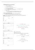
EXAMPLE: Is there a statistically significant difference between number of TV appearances for MPs of different parties?
Figure 1. Number of TV show entries
Figure 2. Total sum of squares (990 ) | 990 = 991 + 992
6
990 = ∑7
389;<3 − <̅4)*,5 >
<̅4)*,5 = 3 + 2 + 4 + 7 + 5 + 6 + 8 + 5 + 7 = 47 ÷ 9 = 5.22
990 = (3 − 5.22)6 + (2 − 5.22)6 + (4 − 5.22)6
+(7 − 5.22)6 + (5 − 5.22)6 + (6 − 5.22)6
+(8 − 5.22)6 + (5 − 5.22)6 + (7 − 5.22)6 = 31.55
FF: = GH. II
Figure 3. Model sum of squares (991 ) - 99;$(<$$,
CDA: <̅9 = (3 + 2 + 4) ÷ 3 = 3
VVD: <̅6 = (7 + 5 + 6) ÷ 3 = 6
PvdA: <̅= = (8 + 5 + 7) ÷ 3 = 6.67
(With k for the group (here: political party) and <̅ > the mean for that group
>
6
991 = J +> ;<̅> − <̅4)*,5 >
>89
= 3(3 − 5.22)6 + 3(6 − 5.22)6 + 3(6.67 − 5.22)6 = 22.89
FF? = KK. LM
Figure 4. Residual sum of squares (992 ) - 99@3(A3,
992 = ∑(<3> − <̅> )6
= (3 − 3)6 + (2 − 3)6 + (4 − 3)6
+(7 − 6)6 + (5 − 6)6 + (6 − 6)6
+(8 − 6.67)6 + (5 − 6.67)6 + (7 − 6.67)6 = 8.67
FFB = L. NO
,991 is good to answer the question: Which part of the total sum of squares can we explain by using the group means?
992 is good to answer the question: Which part of the total sum of squares cannot be explained by using the group means?
Mean squares
• The model sum of squares (991 ) is based on the difference between 3 group means and the grand mean.
o The degrees of freedom is the number of groups minus 1 for the grand mean
991 22.89
P91 = = = 11.44
671 2
671 = 3 − 1 = 2
• The residual sum of squares (992 ) is based on the difference between each value and its group mean
o The degrees of freedom is based on the number of observations (minus the number of groups)
992 8.67
P92 = = = 1.44
672 6
672 = 9 − 3 = 6
F statistic
• The ratio between the variance explained by the model (P91 ) and the variance NOT explained by the model (P92 )
• If Q > 1, the model can explain more than what it leaves unexplained
P91 11.44
Q= = = 7.92
P92 1.44
Inference: conclusion about population
Null hypothesis: the mean of all groups is the same
We compare this score for the F-test to the F-distribution.
This distribution has two sets of degrees of freedom: 671 and 672 . Here: 2 and 6.
Critical value for a significance level (a-level) of 0.05 and 2 and 6 degrees of freedom is 5.14.
SCDEFECGH compared to SIJKLDMLN
• The observed value of F (Q.O#$)P$5 = 7.92) is greater than the correspond ding critical value (Q-)3(3-*/ = 5.14)
• Therefore, we reject the null hypothesis (null hypothesis: the mean of all groups is the same)
Reporting: There was a statistically significant difference (at the 5% level) between parties in terms of the average number of tv show entries by their
politicians, F(2, 6) = 7.92, p = 0.021.
,REGRESSION ANALYSIS
Why do we use regression for statistical inference?
• To express uncertainty about our conclusions about the relation between 2 concepts
• Assessing the strength of a relation
• Understand the population (based on a sample)
Why regression?
• What if we are not just interested in the difference between two means, but in how the mean values of a variable change as another
variable changes
• Example: Have available incomes increased in rich and poor countries, or have poor countries remained poor?
• How can we describe the strength of this association? Correlation? r = 0.961
Regression is related to correlation
• But regression can assess the impact of several independent variables on one specific dependent variable
o Not just strength of the association, but size of the effect: the expected change in Y as a result of a 1-unit change in X
• By assuming a linear association exists
• Regression can assess the null hypothesis: incomes are unrelated to incomes in the past
EXAMPLE: What is the relationship between the number of seats a party has in parliament and the number of motions it tables?
‘Line of best fit’
• Minimizing the distances between points and the line; your best guess given the data available
REGRESSION EQUATION: T = U + V<
• Intercept (constant): a; if the number of seats is 0, how many motions can we expect (according to the model)?
• Slope: b; if the number of seats increases by 1, what is the expected change in the number of motions (according to the model)?
Intercept: Slope:
• If a party has 30 seats, how many motions can we expect?
o W2%X2+5 = U + V ∗ 5ZU%5
o W2%X2+5 = 38.11 + 7.17 ∗ 5ZU%5
o \ = 38.11 + 7.17 ∗ 30 = 253.3
W2%[2+5
• We often use VQ and V9 instead of use U and V
o T3 = VQ + V9 <3
o The subscript X stands for the number of the observation,
T9 is the value of the response variable T for the first observation in the dataset,
T3 is the value of the response variable T for any observation X in the dataset.
ERROR: There are observations not on the regression line, there is error! All models are wrong
, Including error in the equation
• T3 = VQ + V9 <3 + ]3 | All models are wrong, but we make assumptions about error (e.g. it is random for all cases)
• Ε[T3 |<3 ] = VQ + V9 <3 | That’s why we work with the expected value of T3 given a value of bE
HOW DO WE DRAW THE REGRESSION LINE?
• Ordinary Least Squares: Minimizes the residual sum of squares; a residual is the difference between a data point and the regression line
• Squaring these residuals gives us squared residuals, or squares; the sum of the squared residuals is 992 = 24680.2
• The regression line is chosen in such a way that the residual sum of squares is as small as possible, least squares
Calculating the regression line
• 992 = ∑(T3 − Tc3 )6
• 992 = ∑(T3 − VQ − V9 <3 )6
• Tc3 = VQ − V9 <3 ; Tc3 refers to the predicted value of y according to the regression model
Analyze > Correlate > Bivariate > Select Options > Cross-
product deviations and covariances
eR (predicted/estimated dR ) in our example
d
∑(<3 − <̅ )(T3 − Tg) 25908
Vf9 = = = 7.17
(<3 − <̅ )6 3612
Vf9 = 7.17
eS (predicted/estimated dS ) in our example
d
h
VQ = Tg − Vf9 <̅
hQ = 199.5 − 7.17 ∗ 22.5 = 38.17
V
h
VQ = 38.17
Multiple explanatory variables: If you have more than one explanatory variable in your model,
you can still calculate the ‘least squares’, this is what SPSS is for!
Regression: Key assumptions
1. It makes sense to treat the relationship between Ε[T3 |<3 ] and the x variable as linear and additive
2. Ε[T3 |<3 ] = 0, error exists but is assumed to be random, so not relevant for estimating point-values
T3 = VQ + V9 <3 + ]3
Ε[T3 |<3 ] = VQ + V9 <3
What variables are suitable for regression?
• Dependent variable: Interval-ratio scale response variables
o Must have the same substantive meaning anywhere on the scale, e.g. profit, GDP
• Otherwise, modification is needed:
o Nominal/Ordinal scale: Logistic regression (blue/brown, agree, strongly agree)
o Count scale (non-negative integers): Poisson and negative binomial regression models; NOT in this course (war casualties)
• Explanatory variables can be of any type (with modification)
• Variable values must vary (variance cannot be zero)
1. Hypothesis
a. Null hypothesis: ∆= 0
b. Alternative hypothesis: ∆≠ 0
2. Test statistic
"
∆
a. T-test: % = " in this example %̂ = 3.45
%(∆)
#$
3. Sampling distribution of the test statistic
a. T-distribution with 11202 (+()$*(+$,( + +-.,()./ − 2 012345) degrees of freedom
4. Look up/calculate p=value for %̂ = 3.45; 67 = 11202
a. p=0.0006
5. Conclusion
a. Reject the null hypothesis at the 5% significance level (because p < 0.05)
b. Earnings are different from those who followed the training program
II. ANOVA: Comparing more than two means
• If we want to compare more than two means, we cannot use a simple t-test
• ANOVA considers the differences between groups and the differences within groups
EXAMPLE: Is there a statistically significant difference between number of TV appearances for MPs of different parties?
Figure 1. Number of TV show entries
Figure 2. Total sum of squares (990 ) | 990 = 991 + 992
6
990 = ∑7
389;<3 − <̅4)*,5 >
<̅4)*,5 = 3 + 2 + 4 + 7 + 5 + 6 + 8 + 5 + 7 = 47 ÷ 9 = 5.22
990 = (3 − 5.22)6 + (2 − 5.22)6 + (4 − 5.22)6
+(7 − 5.22)6 + (5 − 5.22)6 + (6 − 5.22)6
+(8 − 5.22)6 + (5 − 5.22)6 + (7 − 5.22)6 = 31.55
FF: = GH. II
Figure 3. Model sum of squares (991 ) - 99;$(<$$,
CDA: <̅9 = (3 + 2 + 4) ÷ 3 = 3
VVD: <̅6 = (7 + 5 + 6) ÷ 3 = 6
PvdA: <̅= = (8 + 5 + 7) ÷ 3 = 6.67
(With k for the group (here: political party) and <̅ > the mean for that group
>
6
991 = J +> ;<̅> − <̅4)*,5 >
>89
= 3(3 − 5.22)6 + 3(6 − 5.22)6 + 3(6.67 − 5.22)6 = 22.89
FF? = KK. LM
Figure 4. Residual sum of squares (992 ) - 99@3(A3,
992 = ∑(<3> − <̅> )6
= (3 − 3)6 + (2 − 3)6 + (4 − 3)6
+(7 − 6)6 + (5 − 6)6 + (6 − 6)6
+(8 − 6.67)6 + (5 − 6.67)6 + (7 − 6.67)6 = 8.67
FFB = L. NO
,991 is good to answer the question: Which part of the total sum of squares can we explain by using the group means?
992 is good to answer the question: Which part of the total sum of squares cannot be explained by using the group means?
Mean squares
• The model sum of squares (991 ) is based on the difference between 3 group means and the grand mean.
o The degrees of freedom is the number of groups minus 1 for the grand mean
991 22.89
P91 = = = 11.44
671 2
671 = 3 − 1 = 2
• The residual sum of squares (992 ) is based on the difference between each value and its group mean
o The degrees of freedom is based on the number of observations (minus the number of groups)
992 8.67
P92 = = = 1.44
672 6
672 = 9 − 3 = 6
F statistic
• The ratio between the variance explained by the model (P91 ) and the variance NOT explained by the model (P92 )
• If Q > 1, the model can explain more than what it leaves unexplained
P91 11.44
Q= = = 7.92
P92 1.44
Inference: conclusion about population
Null hypothesis: the mean of all groups is the same
We compare this score for the F-test to the F-distribution.
This distribution has two sets of degrees of freedom: 671 and 672 . Here: 2 and 6.
Critical value for a significance level (a-level) of 0.05 and 2 and 6 degrees of freedom is 5.14.
SCDEFECGH compared to SIJKLDMLN
• The observed value of F (Q.O#$)P$5 = 7.92) is greater than the correspond ding critical value (Q-)3(3-*/ = 5.14)
• Therefore, we reject the null hypothesis (null hypothesis: the mean of all groups is the same)
Reporting: There was a statistically significant difference (at the 5% level) between parties in terms of the average number of tv show entries by their
politicians, F(2, 6) = 7.92, p = 0.021.
,REGRESSION ANALYSIS
Why do we use regression for statistical inference?
• To express uncertainty about our conclusions about the relation between 2 concepts
• Assessing the strength of a relation
• Understand the population (based on a sample)
Why regression?
• What if we are not just interested in the difference between two means, but in how the mean values of a variable change as another
variable changes
• Example: Have available incomes increased in rich and poor countries, or have poor countries remained poor?
• How can we describe the strength of this association? Correlation? r = 0.961
Regression is related to correlation
• But regression can assess the impact of several independent variables on one specific dependent variable
o Not just strength of the association, but size of the effect: the expected change in Y as a result of a 1-unit change in X
• By assuming a linear association exists
• Regression can assess the null hypothesis: incomes are unrelated to incomes in the past
EXAMPLE: What is the relationship between the number of seats a party has in parliament and the number of motions it tables?
‘Line of best fit’
• Minimizing the distances between points and the line; your best guess given the data available
REGRESSION EQUATION: T = U + V<
• Intercept (constant): a; if the number of seats is 0, how many motions can we expect (according to the model)?
• Slope: b; if the number of seats increases by 1, what is the expected change in the number of motions (according to the model)?
Intercept: Slope:
• If a party has 30 seats, how many motions can we expect?
o W2%X2+5 = U + V ∗ 5ZU%5
o W2%X2+5 = 38.11 + 7.17 ∗ 5ZU%5
o \ = 38.11 + 7.17 ∗ 30 = 253.3
W2%[2+5
• We often use VQ and V9 instead of use U and V
o T3 = VQ + V9 <3
o The subscript X stands for the number of the observation,
T9 is the value of the response variable T for the first observation in the dataset,
T3 is the value of the response variable T for any observation X in the dataset.
ERROR: There are observations not on the regression line, there is error! All models are wrong
, Including error in the equation
• T3 = VQ + V9 <3 + ]3 | All models are wrong, but we make assumptions about error (e.g. it is random for all cases)
• Ε[T3 |<3 ] = VQ + V9 <3 | That’s why we work with the expected value of T3 given a value of bE
HOW DO WE DRAW THE REGRESSION LINE?
• Ordinary Least Squares: Minimizes the residual sum of squares; a residual is the difference between a data point and the regression line
• Squaring these residuals gives us squared residuals, or squares; the sum of the squared residuals is 992 = 24680.2
• The regression line is chosen in such a way that the residual sum of squares is as small as possible, least squares
Calculating the regression line
• 992 = ∑(T3 − Tc3 )6
• 992 = ∑(T3 − VQ − V9 <3 )6
• Tc3 = VQ − V9 <3 ; Tc3 refers to the predicted value of y according to the regression model
Analyze > Correlate > Bivariate > Select Options > Cross-
product deviations and covariances
eR (predicted/estimated dR ) in our example
d
∑(<3 − <̅ )(T3 − Tg) 25908
Vf9 = = = 7.17
(<3 − <̅ )6 3612
Vf9 = 7.17
eS (predicted/estimated dS ) in our example
d
h
VQ = Tg − Vf9 <̅
hQ = 199.5 − 7.17 ∗ 22.5 = 38.17
V
h
VQ = 38.17
Multiple explanatory variables: If you have more than one explanatory variable in your model,
you can still calculate the ‘least squares’, this is what SPSS is for!
Regression: Key assumptions
1. It makes sense to treat the relationship between Ε[T3 |<3 ] and the x variable as linear and additive
2. Ε[T3 |<3 ] = 0, error exists but is assumed to be random, so not relevant for estimating point-values
T3 = VQ + V9 <3 + ]3
Ε[T3 |<3 ] = VQ + V9 <3
What variables are suitable for regression?
• Dependent variable: Interval-ratio scale response variables
o Must have the same substantive meaning anywhere on the scale, e.g. profit, GDP
• Otherwise, modification is needed:
o Nominal/Ordinal scale: Logistic regression (blue/brown, agree, strongly agree)
o Count scale (non-negative integers): Poisson and negative binomial regression models; NOT in this course (war casualties)
• Explanatory variables can be of any type (with modification)
• Variable values must vary (variance cannot be zero)