Automata, language theory and complexity
(2IT90) Summary Q1 2020
Any references to figures in this summary are towards the book Introduction to the Theory of Computation
2021 by Michael Sipser.
Chapter 0 Introduction
Read my summaries of the two courses Logic and Set Theory (2IT60) and Discrete Structures (2IT80).
Chapter 1 Regular Languages
A computational model is an idealized computer that is used to simulate mathematical theory.
§1.1: The finite state machine/finite automaton is the simplest computational model.
It is explained using the example of an automatic door that has sensors on both sides of the door. Its state
diagram can be found in figure 1.2 on page 32 and its state transition table can be found in figure 1.3 on
page 33. The probabilistic counterpart of a finite automaton is called a Markov chain. In figure 1.4 on page
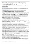
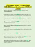
34, we can see a finite automaton. It has three states (𝑞1 , 𝑞2 , 𝑞3 ). The start state 𝑞1 is indicated b the
arrow pointing at it from nowhere. The accept/final state 𝑞2 is indicated by a double circle. The arrows
going from one state to another are called transitions. When this automaton receives an input string, it
processes that string and produces an output: accept (end in accept state) or reject (don’t end there).
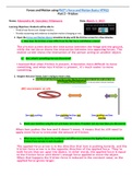
Definition 1.5: A finite automaton is a 5-tuple (𝑄, Σ, 𝛿, 𝑞0 , 𝐹), where
1. 𝑄 is a finite set called the states; 2. Σ is a finite set called the alphabet;
3. 𝛿: 𝑄 × Σ ⟶ 𝑄 is the transition function; 4. 𝑞0 is the start state;
5. 𝐹 ⊆ 𝑄 is the set of accept states.
The transition function defines the rules for moving e.g. from state x to state y if input is 1: 𝛿(𝑥, 1) = 𝑦. We
can define figure 3 now formally: 1. 𝑄 = {𝑞1 , 𝑞2 , 𝑞3 }; 2. Σ = {0,1}; 3. 𝛿 is:
4. 𝑞1 is the start state; 5. 𝐹 = {𝑞2 }.
If 𝐴 is the set of all strings that machine 𝑀 accepts, we say that 𝐴 is the language of machine M
and write 𝐿(𝑀) = 𝐴. We say that 𝑀 recognizes 𝐴 or that 𝑀 accepts 𝐴. A machine may accept several strings
but always recognizes only one language. If accept no strings, it accepts empty language ∅.
Describing a finite automaton by state diagram is not possible in some cases when the diagram would be
too big to draw or if it depends on some unspecified parameter. Then, the formal description is used.
Formal definition of computation: Let 𝑀 = (𝑄, Σ, 𝛿, 𝑞0 , 𝐹) be a finite automaton and let 𝑤 = 𝑤1 𝑤2 ⋯ 𝑤𝑛 be
a string where each 𝑤𝑖 is a member of the alphabet Σ. Then 𝑀 accepts 𝑤 if a sequence of states 𝑟0 , 𝑟1 , … , 𝑟𝑛
in 𝑄 exists with three conditions: 1. 𝑟0 = 𝑞0; 2. 𝛿(𝑟𝑖 , 𝑤𝑖+1 ) = 𝑟𝑖+1 for 𝑖 = 0, … , 𝑛 − 1; 3. 𝑟𝑛 ∈ 𝐹.
i.e. 1. We start in the start state; 2. It goes according to the transition function; 3. We end in an accept state.
Definition 1.16: A language is called a regular language if some finite automaton recognizes it.
Designing finite automata can be done by “pretending to be the machine”. You receive an input string
and must determine after every symbol if the string so far is in the language: you must always be ready with
an answer as you don’t know when the end of the string is. An example is in the book with odd and even.
Definition 1.23: Let 𝐴 and 𝐵 be languages. We define the regular operations union, concatenation and star
as follows: ● Union: 𝐴 ∪ 𝐵 = { 𝑥 | 𝑥 ∈ 𝐴 𝑜𝑟 𝑥 ∈ 𝐵}; ● Concatenation: 𝐴 ∘ 𝐵 = { 𝑥𝑦 | 𝑥 ∈ 𝐴 𝑎𝑛𝑑 𝑦 ∈ 𝐵}
● Star: 𝐴∗ = {𝑥1 𝑥2 … 𝑥𝑘 | 𝑘 ≥ 0 𝑎𝑛𝑑 𝑒𝑎𝑐ℎ 𝑥𝑖 ∈ 𝐴 }.
i.e. The union operation takes all strings in A and B and puts them in one language. The concatenation
operation attaches a string from A in front of a string from B. The star operation is a unary operation
(instead of binary) and attaches any number of strings in A together to get a string in the new language.
“Any number” also includes 0 so 𝐴∗ always includes the empty string 𝜀.
Generally speaking, a collection of objects is closed under some operation if applying that operation to
members of the collection returns an object still in the collection. The collection of regular languages is
closed under all three of the regular operations.
1
Automata (2IT90) Summary Q1 2020 by Isabel Rutten
,Theorem 1.25: The class of regular language is closed under the union operation.
i.e. if 𝐴1 and 𝐴2 are regular languages, so is 𝐴1 ∪ 𝐴2 .
Proof: Because 𝐴1 and 𝐴2 are regular, we know that some finite automaton 𝑀1 recognizes 𝐴1 and some
finite automaton 𝑀2 recognizes 𝐴2 . To prove that 𝐴1 ∪ 𝐴2 is regular, we do a proof by construction by
constructing a finite automaton 𝑀 from 𝑀1 and 𝑀2 that recognizes 𝐴1 ∪ 𝐴2 . This can be done by taking the
Cartesian product 𝑄1 × 𝑄2 of sets 𝑄1 and 𝑄2 for the states.
Theorem 1.26: The class of regular languages is closed under the concatenation operation.
i.e. if 𝐴1 and 𝐴2 are regular languages, so is 𝐴1 ∘ 𝐴2 .
Proof: 𝑀1 recognizes 𝐴1 , 𝑀2 recognizes 𝐴2 . It must accept if its input can be broken into two pieces, where
𝑀1 accepts the first piece and 𝑀2 accepts the second piece. Problem: 𝑀 doesn’t know where to break its
input. To solve this, we use nondeterminism.
§1.2: For a deterministic computation, when the state and next input symbol are given, the next state is
known. In a nondeterministic computation, several choices may exist for the next state at any point.
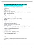
The difference between a deterministic finite automaton, DFA, and a nondeterministic finite automaton,
NFA (fig. 1.27, page 48), is apparent: ● Every state of a DFA always has exactly 1 exiting transition arrow
for each symbol in the alphabet. In an NFA, a state may have 0, 1, or many exiting arrows for each
alphabet symbol.
● In a DFA, labels on the transition arrows are symbols from the alphabet. An NFA may have 0, 1 or many
arrows labeled with members of the alphabet or 𝜀.
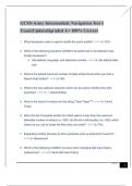
An NFA computes by reading each symbol and if there are multiple options, the machine splits into
multiple copies of itself and follows all possibilities in parallel. This continues recursively. Finally, if any one
of these copies of the machines is in an accept state at the end of the input, the NFA accepts the input
string. This also holds for 𝜺: without reading any input, the machine splits into multiple copies, one
following each of the exiting 𝜀-labeled arrows and one staying at the current state. This continues
recursively. So, an NFA can be seen as a tree of possibilities while the DFA is a straight line (fig. 1.28,
page 49).
In figures 1.31 and 1.32 on page 51 it is clear that the NFA is way easier to read than its DFA.
A unary alphabet is an alphabet containing only one symbol.
Definition 1.37: A nondeterministic finite automaton is a 5-tuple (𝑄, Σ, 𝛿, 𝑞0 , 𝐹), where
1. 𝑄 is a finite set called the states; 2. Σ is a finite set called the alphabet;
3. 𝛿: 𝑄 × Σε ⟶ 𝑃(𝑄) is the transition function; 4. 𝑞0 ∈ 𝑄 is the start state;
5. 𝐹 ⊆ 𝑄 is the set of accept states.
In an NFA, the transition function takes a state and an input symbol or the empty string and produces the
set of possible next states. For any set we write the power set of 𝑄 𝑃(𝑄) as the collection of all subsets of
𝑄. For any alphabet Σ we write Σ𝜀 to be Σ ∪ {𝜀}.
Formal definition of computation for an NFA: Let 𝑁 = (𝑄, Σ, 𝛿, 𝑞0 , 𝐹) be an NFA and 𝑤 a string over the
alphabet Σ. Then we say that 𝑁 accepts 𝑤 if we can write 𝑤 as 𝑤 = 𝑦1 𝑦2 ⋯ 𝑦𝑛 where each 𝑦𝑖 is a member
of Σ𝜀 and a sequence of states 𝑟0 , 𝑟1 , … , 𝑟𝑛 exists in 𝑄 with three conditions: 1. 𝑟0 = 𝑞0;
2. 𝑟𝑖+1 ∈ 𝛿(𝑟𝑖 , 𝑤𝑖+1 ) for 𝑖 = 0, … , 𝑚 − 1; 3. 𝑟𝑚 ∈ 𝐹.
i.e. 1. Start in the start state; 2. The next state is in the set of allowable states; 3. End in an accept state.
Two machines are equivalent if they recognize the same language.
Theorem 1.39: Every nondeterministic finite automaton has an equivalent deterministic finite automaton.
Proof: Recall the “reader as automaton” strategy for designing finite automata: simulate the NFA and
pretend to be a DFA. If 𝑘 is the number of states in the NFA, it has 2𝑘 subsets of states. Each subset
corresponds to a state in the DFA. We do a proof by construction and construct the correct DFA.
2
Automata (2IT90) Summary Q1 2020 by Isabel Rutten
, Corollary 1.40: A language is regular if and only if some nondeterministic finite automaton recognizes it.
Proof: ⇒: any NFA can be converted into an equivalent DFA (theorem 1.39). So, if an NFA recognizes
some language, so does some DFA, and hence the language is regular.
⇐: If a language is regular, there is a DFA that recognizes it, thus also an equivalent NFA (theorem 1.39).
Theorem 1.45: The class of regular languages is closed under the union operation.
Proof: We have regular languages 𝐴1 and 𝐴2 and want to prove that 𝐴1 ∪ 𝐴2 is regular. NFA 𝑁1 recognizes
𝐴1 , 𝑁2 recognizes 𝐴2 . We do a proof by construction by constructing an NFA 𝑁 from 𝑁1 and 𝑁2 that
recognizes 𝐴1 ∪ 𝐴2 (fig. 1.46, page 59). Machine 𝑁 must accept its input if either 𝑁1 or 𝑁2 accepts this input
and must thus nondeterministically guess which of the two machines accepts the input.
Theorem 1.47: The class of regular languages is closed under the concatenation operation.
Proof: We have regular languages 𝐴1 and 𝐴2 and want to prove that 𝐴1 ○ 𝐴2 is regular. NFA 𝑁1 recognizes
𝐴1 , 𝑁2 recognizes 𝐴2 . We do a proof by construction by constructing an NFA 𝑁 from 𝑁1 and 𝑁2 that
recognizes 𝐴1 ○ 𝐴2 (fig. 1.49, page 61). 𝑁’s start state is the start state of 𝑁1 . The accept states of 𝑁1 have
additional 𝜀 arrows that point to the start state of 𝑁2 i.e. an initial piece of the input has been found. The
accept states of 𝑁 are the accept states of 𝑁2 . So, it accepts when the input can be split into two parts, the
first accepted by 𝑁1 , the second by 𝑁2 .
Theorem 1.49: The class of regular languages is closed under the star operation.
Proof: We have regular language 𝐴1 and want to prove that 𝐴1∗ is regular. NFA 𝑁1 recognizes 𝐴1 . We do a
proof by construction by constructing an NFA 𝑁 from 𝑁1 that recognizes 𝐴1∗ (fig. 1.50, page 62). The
resulting NFA 𝑁 will accept its input whenever it can be broken into several pieces and 𝑁1 accepts each
piece. This can be done by placing additional 𝜀 arrows returning to the start state from the accept states.
Also, 𝑁 must accept 𝜀 which is always a member of 𝐴1∗ . We add a new start state and add an 𝜀 arrow from
this to the original start state.
§1.3: In arithmetic, we can use + and × to build expressions e.g. (5 + 3) × 4. Similarly, we can use the
regular operation to build up expressions describing languages, which are called regular expressions e.g.
(0 ∪ 1)0∗ ). The value of the arithmetic expression is 32. The value of a regular expression is a language.
We dissect the example: symbols 0 and 1 are shorthand for the sets {0} and {1}. 0∗ means any number of
{0}. Concatenation symbol ○ is often implicit (like × in arithmetic). So (0 ∪ 1)0∗ is actually ({0} ∪ {1}) ○ {0}∗.
Definition 1.52: Say that R is a regular expression if R is: 1. 𝑎 for some 𝑎 in the alphabet Σ; 2. 𝜀; 3. ∅;
4. (𝑅1 ∪ 𝑅2 ) where 𝑅1 and 𝑅2 are regular expressions;
5. (𝑅1 ○ 𝑅2 ) where 𝑅1 and 𝑅2 are regular expressions; or 6. (𝑅1∗ ) where 𝑅1 is a regular expression.
Note: Don’t get confused: 𝜀 is language containing only empty string. ∅ is language that contains no strings.
We are in danger of defining the notion of a regular expression in terms of itself which is a circular
definition which would be invalid. However, 𝑅1 and 𝑅2 always are smaller than 𝑅 thus we avoid circularity
and have defined an inductive definition.
We let 𝑅 + be shorthand for 𝑅𝑅 ∗ so at least 1 or more concatenations of 𝑅 whereas 𝑅 ∗ has at least 0.
To distinguish between a regular expression 𝑅 and the language it describes, write 𝐿(𝑅) as its language.
If we let 𝑅 be any regular expression we have the following identities:
● 𝑅 ∪ ∅ = 𝑅: adding the empty language will not change it
● 𝑅 ○ 𝜀 = 𝑅: joining the empty string will not change it
● 𝑅 ∪ 𝜀 may not equal 𝑅 e.g. if 𝑅 = {0}, then 𝐿(𝑅) = {0} but 𝐿(𝑅 ∪ 𝜀) = {0, 𝜀}
● 𝑅 ○ ∅ may not equal 𝑅 e.g. if 𝑅 = {0}, then 𝐿(𝑅) = {0} but 𝐿(𝑅 ○ ∅) = ∅
Elemental objects in a programming language, called tokens, may be described with regular expressions.
Then, systems can generate the lexical analyzer (part of compiler that initially processes input program).
3
Automata (2IT90) Summary Q1 2020 by Isabel Rutten
(2IT90) Summary Q1 2020
Any references to figures in this summary are towards the book Introduction to the Theory of Computation
2021 by Michael Sipser.
Chapter 0 Introduction
Read my summaries of the two courses Logic and Set Theory (2IT60) and Discrete Structures (2IT80).
Chapter 1 Regular Languages
A computational model is an idealized computer that is used to simulate mathematical theory.
§1.1: The finite state machine/finite automaton is the simplest computational model.
It is explained using the example of an automatic door that has sensors on both sides of the door. Its state
diagram can be found in figure 1.2 on page 32 and its state transition table can be found in figure 1.3 on
page 33. The probabilistic counterpart of a finite automaton is called a Markov chain. In figure 1.4 on page
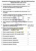
34, we can see a finite automaton. It has three states (𝑞1 , 𝑞2 , 𝑞3 ). The start state 𝑞1 is indicated b the
arrow pointing at it from nowhere. The accept/final state 𝑞2 is indicated by a double circle. The arrows
going from one state to another are called transitions. When this automaton receives an input string, it
processes that string and produces an output: accept (end in accept state) or reject (don’t end there).
Definition 1.5: A finite automaton is a 5-tuple (𝑄, Σ, 𝛿, 𝑞0 , 𝐹), where
1. 𝑄 is a finite set called the states; 2. Σ is a finite set called the alphabet;
3. 𝛿: 𝑄 × Σ ⟶ 𝑄 is the transition function; 4. 𝑞0 is the start state;
5. 𝐹 ⊆ 𝑄 is the set of accept states.
The transition function defines the rules for moving e.g. from state x to state y if input is 1: 𝛿(𝑥, 1) = 𝑦. We
can define figure 3 now formally: 1. 𝑄 = {𝑞1 , 𝑞2 , 𝑞3 }; 2. Σ = {0,1}; 3. 𝛿 is:
4. 𝑞1 is the start state; 5. 𝐹 = {𝑞2 }.
If 𝐴 is the set of all strings that machine 𝑀 accepts, we say that 𝐴 is the language of machine M
and write 𝐿(𝑀) = 𝐴. We say that 𝑀 recognizes 𝐴 or that 𝑀 accepts 𝐴. A machine may accept several strings
but always recognizes only one language. If accept no strings, it accepts empty language ∅.
Describing a finite automaton by state diagram is not possible in some cases when the diagram would be
too big to draw or if it depends on some unspecified parameter. Then, the formal description is used.
Formal definition of computation: Let 𝑀 = (𝑄, Σ, 𝛿, 𝑞0 , 𝐹) be a finite automaton and let 𝑤 = 𝑤1 𝑤2 ⋯ 𝑤𝑛 be
a string where each 𝑤𝑖 is a member of the alphabet Σ. Then 𝑀 accepts 𝑤 if a sequence of states 𝑟0 , 𝑟1 , … , 𝑟𝑛
in 𝑄 exists with three conditions: 1. 𝑟0 = 𝑞0; 2. 𝛿(𝑟𝑖 , 𝑤𝑖+1 ) = 𝑟𝑖+1 for 𝑖 = 0, … , 𝑛 − 1; 3. 𝑟𝑛 ∈ 𝐹.
i.e. 1. We start in the start state; 2. It goes according to the transition function; 3. We end in an accept state.
Definition 1.16: A language is called a regular language if some finite automaton recognizes it.
Designing finite automata can be done by “pretending to be the machine”. You receive an input string
and must determine after every symbol if the string so far is in the language: you must always be ready with
an answer as you don’t know when the end of the string is. An example is in the book with odd and even.
Definition 1.23: Let 𝐴 and 𝐵 be languages. We define the regular operations union, concatenation and star
as follows: ● Union: 𝐴 ∪ 𝐵 = { 𝑥 | 𝑥 ∈ 𝐴 𝑜𝑟 𝑥 ∈ 𝐵}; ● Concatenation: 𝐴 ∘ 𝐵 = { 𝑥𝑦 | 𝑥 ∈ 𝐴 𝑎𝑛𝑑 𝑦 ∈ 𝐵}
● Star: 𝐴∗ = {𝑥1 𝑥2 … 𝑥𝑘 | 𝑘 ≥ 0 𝑎𝑛𝑑 𝑒𝑎𝑐ℎ 𝑥𝑖 ∈ 𝐴 }.
i.e. The union operation takes all strings in A and B and puts them in one language. The concatenation
operation attaches a string from A in front of a string from B. The star operation is a unary operation
(instead of binary) and attaches any number of strings in A together to get a string in the new language.
“Any number” also includes 0 so 𝐴∗ always includes the empty string 𝜀.
Generally speaking, a collection of objects is closed under some operation if applying that operation to
members of the collection returns an object still in the collection. The collection of regular languages is
closed under all three of the regular operations.
1
Automata (2IT90) Summary Q1 2020 by Isabel Rutten
,Theorem 1.25: The class of regular language is closed under the union operation.
i.e. if 𝐴1 and 𝐴2 are regular languages, so is 𝐴1 ∪ 𝐴2 .
Proof: Because 𝐴1 and 𝐴2 are regular, we know that some finite automaton 𝑀1 recognizes 𝐴1 and some
finite automaton 𝑀2 recognizes 𝐴2 . To prove that 𝐴1 ∪ 𝐴2 is regular, we do a proof by construction by
constructing a finite automaton 𝑀 from 𝑀1 and 𝑀2 that recognizes 𝐴1 ∪ 𝐴2 . This can be done by taking the
Cartesian product 𝑄1 × 𝑄2 of sets 𝑄1 and 𝑄2 for the states.
Theorem 1.26: The class of regular languages is closed under the concatenation operation.
i.e. if 𝐴1 and 𝐴2 are regular languages, so is 𝐴1 ∘ 𝐴2 .
Proof: 𝑀1 recognizes 𝐴1 , 𝑀2 recognizes 𝐴2 . It must accept if its input can be broken into two pieces, where
𝑀1 accepts the first piece and 𝑀2 accepts the second piece. Problem: 𝑀 doesn’t know where to break its
input. To solve this, we use nondeterminism.
§1.2: For a deterministic computation, when the state and next input symbol are given, the next state is
known. In a nondeterministic computation, several choices may exist for the next state at any point.
The difference between a deterministic finite automaton, DFA, and a nondeterministic finite automaton,
NFA (fig. 1.27, page 48), is apparent: ● Every state of a DFA always has exactly 1 exiting transition arrow
for each symbol in the alphabet. In an NFA, a state may have 0, 1, or many exiting arrows for each
alphabet symbol.
● In a DFA, labels on the transition arrows are symbols from the alphabet. An NFA may have 0, 1 or many
arrows labeled with members of the alphabet or 𝜀.
An NFA computes by reading each symbol and if there are multiple options, the machine splits into
multiple copies of itself and follows all possibilities in parallel. This continues recursively. Finally, if any one
of these copies of the machines is in an accept state at the end of the input, the NFA accepts the input
string. This also holds for 𝜺: without reading any input, the machine splits into multiple copies, one
following each of the exiting 𝜀-labeled arrows and one staying at the current state. This continues
recursively. So, an NFA can be seen as a tree of possibilities while the DFA is a straight line (fig. 1.28,
page 49).
In figures 1.31 and 1.32 on page 51 it is clear that the NFA is way easier to read than its DFA.
A unary alphabet is an alphabet containing only one symbol.
Definition 1.37: A nondeterministic finite automaton is a 5-tuple (𝑄, Σ, 𝛿, 𝑞0 , 𝐹), where
1. 𝑄 is a finite set called the states; 2. Σ is a finite set called the alphabet;
3. 𝛿: 𝑄 × Σε ⟶ 𝑃(𝑄) is the transition function; 4. 𝑞0 ∈ 𝑄 is the start state;
5. 𝐹 ⊆ 𝑄 is the set of accept states.
In an NFA, the transition function takes a state and an input symbol or the empty string and produces the
set of possible next states. For any set we write the power set of 𝑄 𝑃(𝑄) as the collection of all subsets of
𝑄. For any alphabet Σ we write Σ𝜀 to be Σ ∪ {𝜀}.
Formal definition of computation for an NFA: Let 𝑁 = (𝑄, Σ, 𝛿, 𝑞0 , 𝐹) be an NFA and 𝑤 a string over the
alphabet Σ. Then we say that 𝑁 accepts 𝑤 if we can write 𝑤 as 𝑤 = 𝑦1 𝑦2 ⋯ 𝑦𝑛 where each 𝑦𝑖 is a member
of Σ𝜀 and a sequence of states 𝑟0 , 𝑟1 , … , 𝑟𝑛 exists in 𝑄 with three conditions: 1. 𝑟0 = 𝑞0;
2. 𝑟𝑖+1 ∈ 𝛿(𝑟𝑖 , 𝑤𝑖+1 ) for 𝑖 = 0, … , 𝑚 − 1; 3. 𝑟𝑚 ∈ 𝐹.
i.e. 1. Start in the start state; 2. The next state is in the set of allowable states; 3. End in an accept state.
Two machines are equivalent if they recognize the same language.
Theorem 1.39: Every nondeterministic finite automaton has an equivalent deterministic finite automaton.
Proof: Recall the “reader as automaton” strategy for designing finite automata: simulate the NFA and
pretend to be a DFA. If 𝑘 is the number of states in the NFA, it has 2𝑘 subsets of states. Each subset
corresponds to a state in the DFA. We do a proof by construction and construct the correct DFA.
2
Automata (2IT90) Summary Q1 2020 by Isabel Rutten
, Corollary 1.40: A language is regular if and only if some nondeterministic finite automaton recognizes it.
Proof: ⇒: any NFA can be converted into an equivalent DFA (theorem 1.39). So, if an NFA recognizes
some language, so does some DFA, and hence the language is regular.
⇐: If a language is regular, there is a DFA that recognizes it, thus also an equivalent NFA (theorem 1.39).
Theorem 1.45: The class of regular languages is closed under the union operation.
Proof: We have regular languages 𝐴1 and 𝐴2 and want to prove that 𝐴1 ∪ 𝐴2 is regular. NFA 𝑁1 recognizes
𝐴1 , 𝑁2 recognizes 𝐴2 . We do a proof by construction by constructing an NFA 𝑁 from 𝑁1 and 𝑁2 that
recognizes 𝐴1 ∪ 𝐴2 (fig. 1.46, page 59). Machine 𝑁 must accept its input if either 𝑁1 or 𝑁2 accepts this input
and must thus nondeterministically guess which of the two machines accepts the input.
Theorem 1.47: The class of regular languages is closed under the concatenation operation.
Proof: We have regular languages 𝐴1 and 𝐴2 and want to prove that 𝐴1 ○ 𝐴2 is regular. NFA 𝑁1 recognizes
𝐴1 , 𝑁2 recognizes 𝐴2 . We do a proof by construction by constructing an NFA 𝑁 from 𝑁1 and 𝑁2 that
recognizes 𝐴1 ○ 𝐴2 (fig. 1.49, page 61). 𝑁’s start state is the start state of 𝑁1 . The accept states of 𝑁1 have
additional 𝜀 arrows that point to the start state of 𝑁2 i.e. an initial piece of the input has been found. The
accept states of 𝑁 are the accept states of 𝑁2 . So, it accepts when the input can be split into two parts, the
first accepted by 𝑁1 , the second by 𝑁2 .
Theorem 1.49: The class of regular languages is closed under the star operation.
Proof: We have regular language 𝐴1 and want to prove that 𝐴1∗ is regular. NFA 𝑁1 recognizes 𝐴1 . We do a
proof by construction by constructing an NFA 𝑁 from 𝑁1 that recognizes 𝐴1∗ (fig. 1.50, page 62). The
resulting NFA 𝑁 will accept its input whenever it can be broken into several pieces and 𝑁1 accepts each
piece. This can be done by placing additional 𝜀 arrows returning to the start state from the accept states.
Also, 𝑁 must accept 𝜀 which is always a member of 𝐴1∗ . We add a new start state and add an 𝜀 arrow from
this to the original start state.
§1.3: In arithmetic, we can use + and × to build expressions e.g. (5 + 3) × 4. Similarly, we can use the
regular operation to build up expressions describing languages, which are called regular expressions e.g.
(0 ∪ 1)0∗ ). The value of the arithmetic expression is 32. The value of a regular expression is a language.
We dissect the example: symbols 0 and 1 are shorthand for the sets {0} and {1}. 0∗ means any number of
{0}. Concatenation symbol ○ is often implicit (like × in arithmetic). So (0 ∪ 1)0∗ is actually ({0} ∪ {1}) ○ {0}∗.
Definition 1.52: Say that R is a regular expression if R is: 1. 𝑎 for some 𝑎 in the alphabet Σ; 2. 𝜀; 3. ∅;
4. (𝑅1 ∪ 𝑅2 ) where 𝑅1 and 𝑅2 are regular expressions;
5. (𝑅1 ○ 𝑅2 ) where 𝑅1 and 𝑅2 are regular expressions; or 6. (𝑅1∗ ) where 𝑅1 is a regular expression.
Note: Don’t get confused: 𝜀 is language containing only empty string. ∅ is language that contains no strings.
We are in danger of defining the notion of a regular expression in terms of itself which is a circular
definition which would be invalid. However, 𝑅1 and 𝑅2 always are smaller than 𝑅 thus we avoid circularity
and have defined an inductive definition.
We let 𝑅 + be shorthand for 𝑅𝑅 ∗ so at least 1 or more concatenations of 𝑅 whereas 𝑅 ∗ has at least 0.
To distinguish between a regular expression 𝑅 and the language it describes, write 𝐿(𝑅) as its language.
If we let 𝑅 be any regular expression we have the following identities:
● 𝑅 ∪ ∅ = 𝑅: adding the empty language will not change it
● 𝑅 ○ 𝜀 = 𝑅: joining the empty string will not change it
● 𝑅 ∪ 𝜀 may not equal 𝑅 e.g. if 𝑅 = {0}, then 𝐿(𝑅) = {0} but 𝐿(𝑅 ∪ 𝜀) = {0, 𝜀}
● 𝑅 ○ ∅ may not equal 𝑅 e.g. if 𝑅 = {0}, then 𝐿(𝑅) = {0} but 𝐿(𝑅 ○ ∅) = ∅
Elemental objects in a programming language, called tokens, may be described with regular expressions.
Then, systems can generate the lexical analyzer (part of compiler that initially processes input program).
3
Automata (2IT90) Summary Q1 2020 by Isabel Rutten