Statistics summary
Week 1: Descriptive statistics for one variable (Part 1) / Describing the association
between two variables (Part 2)
Part 1
Variable = recorded info/characteristic
- Age, weight, BMI, disease (y/n), biol. Sex, income etc.
1) Categorical or qualitative variable: place people into groups/categories.
Nominal: no order based on magnitude or side (place of birth, disease, gender)
Ordinal: rank/order (coffee sized, place in race)
2) Numeric or quantitative variable: recorded numeric quantities. Scale in SPSS
Ratio scale: meaningful ‘0’ ratio (age, weight, income)
Interval scale: non-meaningful ‘0’ (temperature; can go below 0)
- Discrete: inter only (0,1,2,3…) (# people in ER, # births) Are counted
- Continuous: measured on continuous scale (weight, age, income, temp.) Are
measured
Identifiers (student ID) are not true variables.
You can always convert numeric categorical (age child/adult/senior)
Cat. Variables can be recorder using numbers.
Categorical or qualitative variable:
Smoking status Freq. Prop. % shows the
distribute
Never 110 0,55 55%
Past 50 0,25 25%
Current 40 0,20 20%
Total 200 1,00 100%
Bar chart (staafdiagram): prop. y-as, smoking status x-as
Pie chart (cirkeldiagram)
Histogram
Properties of histograms:
1. Quantitative Data
2. No gaps gaps because of missing data or it’s a bar chart
3. Bar width is constant
4. Y-as corresponds to the frequency
Counts y-as, scores x-as
Descriptive statistics
Average – ‘typical’ or ‘middle’ central tendency.
Arithmetic/Sample mean (gemiddelde)
Trimmed mean – mean after removing top/bottom off
Median – middle number (50% below, 50% above). median is often preferred over
the mean in situations where the dataset contains outliers or is not symmetrically
distributed.
o Even number: average of the middle 2
Mode – the most common number
Range: largest number – the smallest number
Variance (sigma): (first data point – mean)2 + (2nd data point – mean)2 + (3rd data point –
mean)2 + (4th data point – mean)2 + (5th data point – mean)2
- Sample variance (s2) = variance / n – 1
, Standard deviation: variance = the average amount of variability in your dataset, how
far each score is from the average
- Sample standard deviation (s) = variance
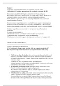
Boxplot
First quartile Q1: 25% below this value
Third quartile Q3: 75% below this value
The box: IQR
Upper fence: Q3 + 1,5*IQR the biggest that is not
an outlier (this doesn’t have to be the maximum)
Lower fence: Q1 – 1,5*IQR the smallest that is
not an outlier (this doesn’t have to be the minimum)
The interquartile range (IQR)= a measure of the
dispersion of a dataset. It is the difference between
Q3 and Q1 and represents the range of the middle
50% of the data. Not sensitive to outliers
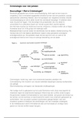
Normal distribution (Gaussian distribution)
Modality
Unimodal: one-peak
Bimodal: two-peaks
Multimodal: two or more peaks
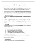
Skewness = (mean- median)/standard deviation
Positively skewed: skewed to the right mode < median
< mean.
Negatively skewed: skewed to the left mean < median
< mode.
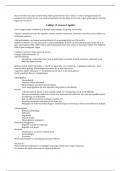
Kurtosis
Leptokurtic: peaks sharply with fat tails less
variability K>0
Mesokurtic: normal distribution/bell shaped
K=0
Week 1: Descriptive statistics for one variable (Part 1) / Describing the association
between two variables (Part 2)
Part 1
Variable = recorded info/characteristic
- Age, weight, BMI, disease (y/n), biol. Sex, income etc.
1) Categorical or qualitative variable: place people into groups/categories.
Nominal: no order based on magnitude or side (place of birth, disease, gender)
Ordinal: rank/order (coffee sized, place in race)
2) Numeric or quantitative variable: recorded numeric quantities. Scale in SPSS
Ratio scale: meaningful ‘0’ ratio (age, weight, income)
Interval scale: non-meaningful ‘0’ (temperature; can go below 0)
- Discrete: inter only (0,1,2,3…) (# people in ER, # births) Are counted
- Continuous: measured on continuous scale (weight, age, income, temp.) Are
measured
Identifiers (student ID) are not true variables.
You can always convert numeric categorical (age child/adult/senior)
Cat. Variables can be recorder using numbers.
Categorical or qualitative variable:
Smoking status Freq. Prop. % shows the
distribute
Never 110 0,55 55%
Past 50 0,25 25%
Current 40 0,20 20%
Total 200 1,00 100%
Bar chart (staafdiagram): prop. y-as, smoking status x-as
Pie chart (cirkeldiagram)
Histogram
Properties of histograms:
1. Quantitative Data
2. No gaps gaps because of missing data or it’s a bar chart
3. Bar width is constant
4. Y-as corresponds to the frequency
Counts y-as, scores x-as
Descriptive statistics
Average – ‘typical’ or ‘middle’ central tendency.
Arithmetic/Sample mean (gemiddelde)
Trimmed mean – mean after removing top/bottom off
Median – middle number (50% below, 50% above). median is often preferred over
the mean in situations where the dataset contains outliers or is not symmetrically
distributed.
o Even number: average of the middle 2
Mode – the most common number
Range: largest number – the smallest number
Variance (sigma): (first data point – mean)2 + (2nd data point – mean)2 + (3rd data point –
mean)2 + (4th data point – mean)2 + (5th data point – mean)2
- Sample variance (s2) = variance / n – 1
, Standard deviation: variance = the average amount of variability in your dataset, how
far each score is from the average
- Sample standard deviation (s) = variance
Boxplot
First quartile Q1: 25% below this value
Third quartile Q3: 75% below this value
The box: IQR
Upper fence: Q3 + 1,5*IQR the biggest that is not
an outlier (this doesn’t have to be the maximum)
Lower fence: Q1 – 1,5*IQR the smallest that is
not an outlier (this doesn’t have to be the minimum)
The interquartile range (IQR)= a measure of the
dispersion of a dataset. It is the difference between
Q3 and Q1 and represents the range of the middle
50% of the data. Not sensitive to outliers
Normal distribution (Gaussian distribution)
Modality
Unimodal: one-peak
Bimodal: two-peaks
Multimodal: two or more peaks
Skewness = (mean- median)/standard deviation
Positively skewed: skewed to the right mode < median
< mean.
Negatively skewed: skewed to the left mean < median
< mode.
Kurtosis
Leptokurtic: peaks sharply with fat tails less
variability K>0
Mesokurtic: normal distribution/bell shaped
K=0