QUAT6221 LU6
QUAT6221 LU6 –Probability Distributions
Chapter 5
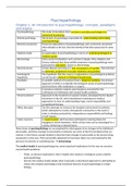
5.1 Intro
Probability distribution = list of all possible outcomes of a random variable and their
associated probabilities of occurrence.
5.2 Types of probability distribution
2 types – depends on the data type of the random variable
1. Discrete
Probability is based on an educated guess, expert opinion or intuition
Probability distribution functions:
- Binomial distribution
- Poisson Distribution
2. Continuous
Probability can be verified statistically
Probability distribution function:
- Normal Distribution
5.3 Discrete Probability Distributions
= assume that the outcomes of a random variable under study can take on only specific
(integer) values
Math’s class can have 1,2,3,4 number of students
Company can have 0,5,10 employees absent on a day
In discrete probability, each outcome has a set chance (not zero) if it’s part of the sample
space. If it’s not part of that space, the chance is zero.
Two common discrete probability distribution functions are binomial (fixed number of
repeated trials) and Poisson (counting events over time or space).
5.4 Binomial Probability Distribution
A discrete random variable follows the binomial distribution if it meets these conditions:
1. The random variable is observed n number of times
2. There are only 2 mutually exclusive and collectively exhaustive outcomes associated
with the random variable on each object in the sample. The 2 outcomes are labelled
success and failure – employee is absent or is not absent
3. Each outcome has an associated probability: success outcome is denoted by p and
failure is denoted by 1-p
4. The objects are assumed to be independent of each other, this means that p is the
same (constant) for each of the n objects.
1
,QUAT6221 LU6
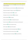
If all 4 conditions are met, the binomial question can be addressed
The binomial question
= “What is the probability that x successes will occur in a randomly drawn sample of n
objects?”
This can be calculated using the binomial probability distribution formula:
❑ x n−x
P ( x )= nC x p ( 1− p) for x = 0,1,2,3,….,n
n = sample size
x = number of success outcomes in the n independently drawn objects
p = probability of a success outcome on a single independent object
(1-p) = probability of a failure outcome on a single independent object
x is also called the domain, since the number of success outcomes cannot exceed the
number of trials, the domain for the BPD is limited to all the integer values (0 – n)
Example 5.1
Zeplin car hire wants to know the chance that 2 out of 5 clients will ask for an Opel. Since 1
in 4 people usually request an Opel, the probability is p = 0.25.
This situation fits a binomial distribution because:
1. There are 5 clients (fixed number of trials).
2. Each client either asks for an Opel (success) or doesn’t (failure).
3. The chance of success (25%) stays the same each time.
4. Each client’s choice is independent.
So, we calculate the binomial probability:
n = 5, x = 2, p = 0.25
Plugged into the binomial formula, the result is 0.264.
There’s a 26.4% chance that exactly 2 out of 5 clients will request an Opel.
How to select p
The success outcome is always associated with the probability p. The outcome that must be
labelled as the success outcome is identified from the binomial question.
Example 5.2
Global Insurance says 20% (1 in 5) of all policies are surrendered before their maturity date.
Assume you randomly pick 10 policies.
This is a binomial distribution because:
1. Fixed number of trials: 10 policies
2. Two outcomes: surrendered or not surrendered
2
, QUAT6221 LU6
3. Constant probability: p = 0.20
4. Trials are independent
(a) What is the probability that 4 of these 10 insurance policies will have been surrendered
before their maturity date?
- random variable is observed 10 times – 10 policies were sampled
- only 2 possible outcomes foreach policy
- a probability can be assigned to each outcome for a policy, namely:
o p = policy surrendered before maturity – success outcome
o p – 1 = policy not surrendered before maturity – failure outcome
- trials are independent, each policy’s status is independent of every other policy’s
status. P= 0.2 is constant for each policy.
Since all conditions for the binomial process have been satisfied, the bionomical
question can be answered
P(x = 4) when n = 10 and p = 0.20
❑ 4 10−4
P ( 4 )=10C 4 p (1− p)
= 0.088 → So there’s an 8.8% chance that exactly 4 of the 10 policies were
surrendered.
(b) What’s the probability that no more than 3 of the 10 policies will have been surrendered
before their maturity date?
“No more than 3” means 0, 1, 2, or 3 surrenders before maturity. We find P(x ≤ 3).
P(x ≤ 3) = P(x=0) + P(x=1) + P(x=2) + P(x=3)
P ( 0 )=1❑0C 0 p 0 (1− p)10−0
P ( 1 )=1❑0C1 p 1 (1− p)10−1
P ( 2 )=10❑C2 p2 (1− p)10−2
P ( 3 )=10❑C 3 p3 (1− p)10−3
P(x ≤ 3) = 0.107 + 0.269 + 0.302+ 0.201 = 0.879 → there’s an 87.9% chance that no
more than 3 of the 10 policies will have been surrendered before their maturity date
(c) What’s the probability that at least 2 of the 10 randomly selected policies will be
surrendered before their maturity date?
P(x ≥ 2) = P(x = 2) + P(x = 3) + P(x = 4) + … + P(x = 10)
P(x ≥ 2) = 1 – P(x ≤ 1) = 0.624
So there’s a 62.4% chance that at least 2 of the 10 randomly selected policies were
surrendered before their maturity rate.
3
QUAT6221 LU6 –Probability Distributions
Chapter 5
5.1 Intro
Probability distribution = list of all possible outcomes of a random variable and their
associated probabilities of occurrence.
5.2 Types of probability distribution
2 types – depends on the data type of the random variable
1. Discrete
Probability is based on an educated guess, expert opinion or intuition
Probability distribution functions:
- Binomial distribution
- Poisson Distribution
2. Continuous
Probability can be verified statistically
Probability distribution function:
- Normal Distribution
5.3 Discrete Probability Distributions
= assume that the outcomes of a random variable under study can take on only specific
(integer) values
Math’s class can have 1,2,3,4 number of students
Company can have 0,5,10 employees absent on a day
In discrete probability, each outcome has a set chance (not zero) if it’s part of the sample
space. If it’s not part of that space, the chance is zero.
Two common discrete probability distribution functions are binomial (fixed number of
repeated trials) and Poisson (counting events over time or space).
5.4 Binomial Probability Distribution
A discrete random variable follows the binomial distribution if it meets these conditions:
1. The random variable is observed n number of times
2. There are only 2 mutually exclusive and collectively exhaustive outcomes associated
with the random variable on each object in the sample. The 2 outcomes are labelled
success and failure – employee is absent or is not absent
3. Each outcome has an associated probability: success outcome is denoted by p and
failure is denoted by 1-p
4. The objects are assumed to be independent of each other, this means that p is the
same (constant) for each of the n objects.
1
,QUAT6221 LU6
If all 4 conditions are met, the binomial question can be addressed
The binomial question
= “What is the probability that x successes will occur in a randomly drawn sample of n
objects?”
This can be calculated using the binomial probability distribution formula:
❑ x n−x
P ( x )= nC x p ( 1− p) for x = 0,1,2,3,….,n
n = sample size
x = number of success outcomes in the n independently drawn objects
p = probability of a success outcome on a single independent object
(1-p) = probability of a failure outcome on a single independent object
x is also called the domain, since the number of success outcomes cannot exceed the
number of trials, the domain for the BPD is limited to all the integer values (0 – n)
Example 5.1
Zeplin car hire wants to know the chance that 2 out of 5 clients will ask for an Opel. Since 1
in 4 people usually request an Opel, the probability is p = 0.25.
This situation fits a binomial distribution because:
1. There are 5 clients (fixed number of trials).
2. Each client either asks for an Opel (success) or doesn’t (failure).
3. The chance of success (25%) stays the same each time.
4. Each client’s choice is independent.
So, we calculate the binomial probability:
n = 5, x = 2, p = 0.25
Plugged into the binomial formula, the result is 0.264.
There’s a 26.4% chance that exactly 2 out of 5 clients will request an Opel.
How to select p
The success outcome is always associated with the probability p. The outcome that must be
labelled as the success outcome is identified from the binomial question.
Example 5.2
Global Insurance says 20% (1 in 5) of all policies are surrendered before their maturity date.
Assume you randomly pick 10 policies.
This is a binomial distribution because:
1. Fixed number of trials: 10 policies
2. Two outcomes: surrendered or not surrendered
2
, QUAT6221 LU6
3. Constant probability: p = 0.20
4. Trials are independent
(a) What is the probability that 4 of these 10 insurance policies will have been surrendered
before their maturity date?
- random variable is observed 10 times – 10 policies were sampled
- only 2 possible outcomes foreach policy
- a probability can be assigned to each outcome for a policy, namely:
o p = policy surrendered before maturity – success outcome
o p – 1 = policy not surrendered before maturity – failure outcome
- trials are independent, each policy’s status is independent of every other policy’s
status. P= 0.2 is constant for each policy.
Since all conditions for the binomial process have been satisfied, the bionomical
question can be answered
P(x = 4) when n = 10 and p = 0.20
❑ 4 10−4
P ( 4 )=10C 4 p (1− p)
= 0.088 → So there’s an 8.8% chance that exactly 4 of the 10 policies were
surrendered.
(b) What’s the probability that no more than 3 of the 10 policies will have been surrendered
before their maturity date?
“No more than 3” means 0, 1, 2, or 3 surrenders before maturity. We find P(x ≤ 3).
P(x ≤ 3) = P(x=0) + P(x=1) + P(x=2) + P(x=3)
P ( 0 )=1❑0C 0 p 0 (1− p)10−0
P ( 1 )=1❑0C1 p 1 (1− p)10−1
P ( 2 )=10❑C2 p2 (1− p)10−2
P ( 3 )=10❑C 3 p3 (1− p)10−3
P(x ≤ 3) = 0.107 + 0.269 + 0.302+ 0.201 = 0.879 → there’s an 87.9% chance that no
more than 3 of the 10 policies will have been surrendered before their maturity date
(c) What’s the probability that at least 2 of the 10 randomly selected policies will be
surrendered before their maturity date?
P(x ≥ 2) = P(x = 2) + P(x = 3) + P(x = 4) + … + P(x = 10)
P(x ≥ 2) = 1 – P(x ≤ 1) = 0.624
So there’s a 62.4% chance that at least 2 of the 10 randomly selected policies were
surrendered before their maturity rate.
3