Use when: 1. Investigating ranking (example: we are checking who arrives first) 2. assumptions not met (Shapiro wilk and levine etc.) (especially normality or both normality and equal variance) 3. small sample size
Non-parametric tests Hypothesis Calculate In R Interpretation
Wilcoxon signed-rank test - 1 sample (1 group) or 2 H0: medians are ‘the Check, timewise (future – the past) do you need a new sample? (F.e.: The research #1 change = data510$t2 - data510$t1 wilcox.test(change) P-Value = 0.028 < 0.05 so we reject H0 which means
paired samples same’ (not sig. question is: “Did the physical condition of this group of students significantly improve #2 wilcox.test(data510$t2, data510$t1, paired = TRUE) that the medians between t2 and t1 are different. In
(Normally: pre-posttest so 2 ‘samples’ become 1 (the different) within 10 weeks after giving students the exercise program?”) Example output: other words, it means the physical condition has change
difference between the tests/two variables) median(group1) = #1st option: we compute the new sample V = 88, p-value = 0.02801 alternative hypothesis: true location is not equal to 0 after the program. In other words, the program had an
median(group2) #2nd option: without computing new sample effect on physical condition.
HA: Medians are
Mann-Whitney-Wilcoxon test (Wilcoxon rank sum Between two groups (control and treatment groups) wilcox.test(asthma ~ group, data = ex1, paired = FALSE) P-Value = 0.058 > 0.05 so we can’t reject H0.
different
test) – 2 samples (2 groups) NB** -> you can simply write (asthma ~ group, data = ex1) as it will compute by default This means that there is no significant difference in
median(group1) ≠
Wilcoxon rank sum test medians between groups (placebo and control). In that
median(group2)
Example output: specific example it means that the new drug is not really
Wilcoxon rank sum test with continuity correction data: asthma by group W = 22, p-value effective.
OR
= 0.05855 alternative hypothesis: true location shift is not equal to 0
Kruskal-Wallis test – more than 2 samples (for H0: Same (similar) More than 2 samples // not related but no space: kruskal.test(depress ~ type, data = ex4) P-Value < 0.05 so we can reject H0.
example: 3 samples (groups) distributions between Example output: This means that there is a significant difference in
If curve is parabolic its squared. Kruskal-Wallis rank sum test medians of depression between the three groups. In
groups Ratio = squared
HA: different In Q: especially big its squared data: depress by type other words, it means that there is an effect of type of
distributions
When lines overlap X1 (usually) = 0 Kruskal-Wallis chi-squared = 15.741, df = 2, p-value = 0.0003819 exercise on depression (at least 2 variables = p-value)
and not included
**so far we can’t tell which group led to more depression given this output, you can
When 3 categories only use 2 cat. In
equation. (1 is the reference) always create a plot to visualize the different levels of depression
B1x2
residuals not normal = adding omitted var transforming y
Linear equations Question/R Interpretation // When 0 remove from equation, when 1 leave only numbers in.
Effect of two "
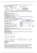
Y(ageism) = β! + β" ∗ Age" + β# ∗ Education# Codes (with and without pipe): Testing the general expectations (whether the Testing specific expectations (For both education and age): t test of b-coefficients
ratio variables " = 𝛃𝟎 + (𝛃𝟏 ∗ 𝑿𝟏 ) + (𝛃𝟐 ∗ 𝑿𝟐 )
𝐘 1. model_name = lm(data_name$ageism ~ data_name$age + model is correct): F test - H0: BETA1 = 0 (age has no effect on ageism)
on a ratio Typical questions: data_name$education) - H0: BETA2= BETA1=0 (Variables have no effect) - HA: BETA1 ≠ 0 (There is a negative effect of age on ageism)
variable Linear equation: Y = 7.257 – 0.088(age) + 0.1077(education) 2. model_name = lm(ageism ~ age + education, data = data_name) - HA: At least one coefficient B is not 0 - H0: BETA2 = 0 (Level of education has no effect on ageism)
(addition) Expected level of ageism (y) for someone who is 30 years old and a 3. model_name = data_name %>% lm(ageism ~ age + education, . ) - H0: The data fits the model - HA: BETA2 ≠ 0 (There is a negative effect of level of education on ageism)
level of education of 5 // Y = 7.257 – 0.088*(30) + 0.1077*(5) = 5,11 summary(model_name) - HA: The data does not fit the model
Calculate a 95% confidence interval for the effect of x1 (age) // Lower:
-0.088 – 2 * 0.0174 = -0.1228 // Upper: -0.088 + 2 * 0.0174 = -0.0532
Effect of a ratio " = β! + β" ∗ Type" + β# ∗ Education#
Y Education dummy coded as (0) = no education, (1) yes education lm(formula = ageism ~ age + edu_dummy, data = A - What is the effect (coefficient) of age on ageism? -> -0.0877
variable and a " = 𝛃𝟎 + (𝛃𝟏 ∗ 𝑿𝟏 ) + (𝛃𝟐 ∗ 𝑿𝟐 )
𝐘 For no education: (x2=0): ass550_clean1) B - What is the expected level of ageism of someone who is 20 years old and had access to
dummy on a ratio y = β0 + β1*x1(age) + β2*0 Coefficients: Estimate Std. Error t value Pr(>|t|) education?
variable y = β0 + β1*x1(age). (Intercept) 7.44552 0.95386 7.806 3.26e-11 *** ▪ Y= 7.44 -0.087(Age) + 0.814(edu_dummy)
(addition) B0 is the intercept and B1 is the slope age -0.08776 0.01730 -5.073 2.88e-06 *** ▪ Y = 7.44 – 0.87(20) + 0.814(1) = 6.14
For yes education: (x2 = 1) edu_dummy 0.81478 0.64786 1.258 0.213 C - What is the expected level of ageism of someone who is 40 years old and no access to
y = β0 + β1*x1(age) + β2*1 General linear equation: y = 7.44 -0.087(age) + education?
y = (β 0+ β 2) + β1*x1(age). 0.814 (edu_dummy) ▪ Y= 7.44 -0.087(Age) + 0.814(edu_dummy)
(β 0+ β2) is the intercept and B1 is the slope (b-coefficent) ▪ Y = 7.44 – 0.87(40) + 0.814(0) = 3.96
effect: (no intercept)
Effect of a ratio The effect of a variable (campaign) can be different for different groups
variable and two (high or low education)
dummy variables Linear equation for high educated (x2=1)
(interaction) y = β0 + β1*x1(campaign) + β2*1- β3*x1*1
y = (β0 + β2) + (β1- β3)*x1(campaign) o where: (β0 + β2) is the intercept
and (β1- β3) is the slope (b-coefficient)
Linear equation for low educated (x2=0)
y = β0 + β1*x1(campaign) + β2*0 - β3*x1*0
y = β0+ β1x1(campaign) o where: β0 is the intercept and β1 is the slope
(Y)= β0 + β1 * x1(campaign) + β2 * x2(education) + (b-coefficient)
β3*x1*x2(Interaction)
Effect of a ratio 𝐼𝑛𝑐𝑜𝑚𝑒 = 𝛽# + 𝛽" 𝐺𝑒𝑛𝑑𝑒𝑟" + (𝛽# ∗ 𝐸𝑑𝑢𝑐𝑎𝑡𝑖𝑜𝑛2) + (𝛽' ∗ 𝐺𝑒𝑛𝑑𝑒𝑟" What is the expected income (scale) of an employee who has 10 years Y = B0 + B1x(scale) + B2x(dummy) + B3x(scale)*x2(dummy), where:
variable and a ∗ 𝐸𝑑𝑢𝑐𝑎𝑡𝑖𝑜𝑛# ) of experience (scale) and a master degree (dummy)? Y = 1115 + 181(10) - B0 Value of the intercept (reference)
dummy on a ratio 𝐘 = 𝜷𝟎 + 𝜷𝟏 𝑿𝟏 + (𝜷𝟐 ∗ 𝑿𝟐 ) + (𝜷𝟑 ∗ 𝑿𝟏 ∗ 𝑿𝟐 ) + 614(1) + 6*(10)*(1) = 3599 - B0 = When x=0, Y = ?
variable B3 = education:campaign Y = income + experience*(10 years) + master*(1=yes) + effect - B1 Value of the b-coefficient associated with the variable “x” (slope for the reference category (group 1))
(interaction) Correct: A high (and significant) F value means that the model experience:master = 6 *(10 years) * (1 = yes) = 3599 - B1 = When x increases by 1, y decreases by 1 (difference y (- each other) / difference x (- each other))
estimated here is correct. - B2 = Value of the b-coefficient associated with the group variable (the dummy) (represents the difference between the lines)
Incorrect: The p-value associated with X1 (<0.05) is smaller than the p- - B2 = Difference between lines (group-reference) when x=0.
value associated with X2 (>0.05). This is because the estimate (see - B3 Value of the b-coefficient associated with the interaction (represents the interaction)
output) of X1(-0.09) is larger (in absolute terms) than X2 (-0.06). - B3 = Difference btw lines when x increases by 1. Must: Start at the intersection, then think group – reference (Note: + if group above – if under)
Non-parametric tests Hypothesis Calculate In R Interpretation
Wilcoxon signed-rank test - 1 sample (1 group) or 2 H0: medians are ‘the Check, timewise (future – the past) do you need a new sample? (F.e.: The research #1 change = data510$t2 - data510$t1 wilcox.test(change) P-Value = 0.028 < 0.05 so we reject H0 which means
paired samples same’ (not sig. question is: “Did the physical condition of this group of students significantly improve #2 wilcox.test(data510$t2, data510$t1, paired = TRUE) that the medians between t2 and t1 are different. In
(Normally: pre-posttest so 2 ‘samples’ become 1 (the different) within 10 weeks after giving students the exercise program?”) Example output: other words, it means the physical condition has change
difference between the tests/two variables) median(group1) = #1st option: we compute the new sample V = 88, p-value = 0.02801 alternative hypothesis: true location is not equal to 0 after the program. In other words, the program had an
median(group2) #2nd option: without computing new sample effect on physical condition.
HA: Medians are
Mann-Whitney-Wilcoxon test (Wilcoxon rank sum Between two groups (control and treatment groups) wilcox.test(asthma ~ group, data = ex1, paired = FALSE) P-Value = 0.058 > 0.05 so we can’t reject H0.
different
test) – 2 samples (2 groups) NB** -> you can simply write (asthma ~ group, data = ex1) as it will compute by default This means that there is no significant difference in
median(group1) ≠
Wilcoxon rank sum test medians between groups (placebo and control). In that
median(group2)
Example output: specific example it means that the new drug is not really
Wilcoxon rank sum test with continuity correction data: asthma by group W = 22, p-value effective.
OR
= 0.05855 alternative hypothesis: true location shift is not equal to 0
Kruskal-Wallis test – more than 2 samples (for H0: Same (similar) More than 2 samples // not related but no space: kruskal.test(depress ~ type, data = ex4) P-Value < 0.05 so we can reject H0.
example: 3 samples (groups) distributions between Example output: This means that there is a significant difference in
If curve is parabolic its squared. Kruskal-Wallis rank sum test medians of depression between the three groups. In
groups Ratio = squared
HA: different In Q: especially big its squared data: depress by type other words, it means that there is an effect of type of
distributions
When lines overlap X1 (usually) = 0 Kruskal-Wallis chi-squared = 15.741, df = 2, p-value = 0.0003819 exercise on depression (at least 2 variables = p-value)
and not included
**so far we can’t tell which group led to more depression given this output, you can
When 3 categories only use 2 cat. In
equation. (1 is the reference) always create a plot to visualize the different levels of depression
B1x2
residuals not normal = adding omitted var transforming y
Linear equations Question/R Interpretation // When 0 remove from equation, when 1 leave only numbers in.
Effect of two "
Y(ageism) = β! + β" ∗ Age" + β# ∗ Education# Codes (with and without pipe): Testing the general expectations (whether the Testing specific expectations (For both education and age): t test of b-coefficients
ratio variables " = 𝛃𝟎 + (𝛃𝟏 ∗ 𝑿𝟏 ) + (𝛃𝟐 ∗ 𝑿𝟐 )
𝐘 1. model_name = lm(data_name$ageism ~ data_name$age + model is correct): F test - H0: BETA1 = 0 (age has no effect on ageism)
on a ratio Typical questions: data_name$education) - H0: BETA2= BETA1=0 (Variables have no effect) - HA: BETA1 ≠ 0 (There is a negative effect of age on ageism)
variable Linear equation: Y = 7.257 – 0.088(age) + 0.1077(education) 2. model_name = lm(ageism ~ age + education, data = data_name) - HA: At least one coefficient B is not 0 - H0: BETA2 = 0 (Level of education has no effect on ageism)
(addition) Expected level of ageism (y) for someone who is 30 years old and a 3. model_name = data_name %>% lm(ageism ~ age + education, . ) - H0: The data fits the model - HA: BETA2 ≠ 0 (There is a negative effect of level of education on ageism)
level of education of 5 // Y = 7.257 – 0.088*(30) + 0.1077*(5) = 5,11 summary(model_name) - HA: The data does not fit the model
Calculate a 95% confidence interval for the effect of x1 (age) // Lower:
-0.088 – 2 * 0.0174 = -0.1228 // Upper: -0.088 + 2 * 0.0174 = -0.0532
Effect of a ratio " = β! + β" ∗ Type" + β# ∗ Education#
Y Education dummy coded as (0) = no education, (1) yes education lm(formula = ageism ~ age + edu_dummy, data = A - What is the effect (coefficient) of age on ageism? -> -0.0877
variable and a " = 𝛃𝟎 + (𝛃𝟏 ∗ 𝑿𝟏 ) + (𝛃𝟐 ∗ 𝑿𝟐 )
𝐘 For no education: (x2=0): ass550_clean1) B - What is the expected level of ageism of someone who is 20 years old and had access to
dummy on a ratio y = β0 + β1*x1(age) + β2*0 Coefficients: Estimate Std. Error t value Pr(>|t|) education?
variable y = β0 + β1*x1(age). (Intercept) 7.44552 0.95386 7.806 3.26e-11 *** ▪ Y= 7.44 -0.087(Age) + 0.814(edu_dummy)
(addition) B0 is the intercept and B1 is the slope age -0.08776 0.01730 -5.073 2.88e-06 *** ▪ Y = 7.44 – 0.87(20) + 0.814(1) = 6.14
For yes education: (x2 = 1) edu_dummy 0.81478 0.64786 1.258 0.213 C - What is the expected level of ageism of someone who is 40 years old and no access to
y = β0 + β1*x1(age) + β2*1 General linear equation: y = 7.44 -0.087(age) + education?
y = (β 0+ β 2) + β1*x1(age). 0.814 (edu_dummy) ▪ Y= 7.44 -0.087(Age) + 0.814(edu_dummy)
(β 0+ β2) is the intercept and B1 is the slope (b-coefficent) ▪ Y = 7.44 – 0.87(40) + 0.814(0) = 3.96
effect: (no intercept)
Effect of a ratio The effect of a variable (campaign) can be different for different groups
variable and two (high or low education)
dummy variables Linear equation for high educated (x2=1)
(interaction) y = β0 + β1*x1(campaign) + β2*1- β3*x1*1
y = (β0 + β2) + (β1- β3)*x1(campaign) o where: (β0 + β2) is the intercept
and (β1- β3) is the slope (b-coefficient)
Linear equation for low educated (x2=0)
y = β0 + β1*x1(campaign) + β2*0 - β3*x1*0
y = β0+ β1x1(campaign) o where: β0 is the intercept and β1 is the slope
(Y)= β0 + β1 * x1(campaign) + β2 * x2(education) + (b-coefficient)
β3*x1*x2(Interaction)
Effect of a ratio 𝐼𝑛𝑐𝑜𝑚𝑒 = 𝛽# + 𝛽" 𝐺𝑒𝑛𝑑𝑒𝑟" + (𝛽# ∗ 𝐸𝑑𝑢𝑐𝑎𝑡𝑖𝑜𝑛2) + (𝛽' ∗ 𝐺𝑒𝑛𝑑𝑒𝑟" What is the expected income (scale) of an employee who has 10 years Y = B0 + B1x(scale) + B2x(dummy) + B3x(scale)*x2(dummy), where:
variable and a ∗ 𝐸𝑑𝑢𝑐𝑎𝑡𝑖𝑜𝑛# ) of experience (scale) and a master degree (dummy)? Y = 1115 + 181(10) - B0 Value of the intercept (reference)
dummy on a ratio 𝐘 = 𝜷𝟎 + 𝜷𝟏 𝑿𝟏 + (𝜷𝟐 ∗ 𝑿𝟐 ) + (𝜷𝟑 ∗ 𝑿𝟏 ∗ 𝑿𝟐 ) + 614(1) + 6*(10)*(1) = 3599 - B0 = When x=0, Y = ?
variable B3 = education:campaign Y = income + experience*(10 years) + master*(1=yes) + effect - B1 Value of the b-coefficient associated with the variable “x” (slope for the reference category (group 1))
(interaction) Correct: A high (and significant) F value means that the model experience:master = 6 *(10 years) * (1 = yes) = 3599 - B1 = When x increases by 1, y decreases by 1 (difference y (- each other) / difference x (- each other))
estimated here is correct. - B2 = Value of the b-coefficient associated with the group variable (the dummy) (represents the difference between the lines)
Incorrect: The p-value associated with X1 (<0.05) is smaller than the p- - B2 = Difference between lines (group-reference) when x=0.
value associated with X2 (>0.05). This is because the estimate (see - B3 Value of the b-coefficient associated with the interaction (represents the interaction)
output) of X1(-0.09) is larger (in absolute terms) than X2 (-0.06). - B3 = Difference btw lines when x increases by 1. Must: Start at the intersection, then think group – reference (Note: + if group above – if under)