The Schrodinger Equation
Time Dependent
total energy operator
- T(x ,
t) + VT t) ,
=
it Tr(x t) ,
C FN iM =
TDSE
Im d ↳ -Stax only depends
V =
on c ,
not .
out
-
Kinetic
energy operator Potential energy operator
The momentum operator p -it : =
The Kinetic energy operator F : =
-
The operator representing the total
energy (the Hamiltonian)
H : = + V = -ve
The TDSE is a linear differential equation -
implies that the superposition principle holds : If M and M are solutions,
then AT + BT is also a solution. Thus
given quantum system energy eigen functions (with definite energy
for a ,
as well as superposition states (with simultaneous multiple energies) satisfy the TDSE .
The TDSE time the wave function TG to) at some time to uniquely determines the
is first order in
specifying
-
,
wave function at a later time (if no measurement is taken/the system is unperturbed). Thus the quantum state
evolves deterministically.
Time-Independent
We only consider timeindependent potential energies
-
V(),
so we can write the energy eigenfunction as a
product of a
Spatial and a temporal solution :
↑(x t) u(x) T(t) only the form of not of superposition states
eigenfunctions
=
energy
=
, ,
Inserting this into the TDSE we obtain : - Ub T(t) + Vbc)uk) T(t) =
in ux T(t) (= u() + (t)
Dividing into (C) and (t) terms gives :
- + V
=
Bothsides must be equal to the same constant with units of energy ,
as it must have the same unit as V() -
> E
which denotes the total
energy .
We obtain the TISE
by setting the LHS equal to E and
multiplying by u (x) :
Flu
- u(x) Vu() Enk) or El
=
+ =
The TISE is an
energy eigenvalue equation with energy eigenfunction () and energy eigenvalue E Thus,
, .
only quantum states with definite
energy (zero uncertainty) can solve the TISE (unlike the TDSE which can be
solved by both energy eigenfunctions and superposition states).
We can obtain the temporal solution by the RHS equal to E
setting
-
iEt
and multiplying by Tt)
dT(t) =
-
iET(t) >
-
T(t) = et = temporal solution for any potential energy VGC)
dt h
, Conditions for Quantum Mechanical Wave functions
*
In one dimension the probability density ↑N T N is a probability length with units [m-] . Thus N t)>
per
=
,
is the probability position measurement of the particle in the interval da
,
upon , finding .
·
Normalisation condition : (% 2 dx =
1
Any function f(x) that is square-integrable can be normalised : ( f(x)x = a # f(x) is correctly
A function is
only square-integrable if M t) > 0 as C-10 . normalised
+
,
·
In addition to being normalised ,
a valid wave function must be continuous -
a
discontinuity would lead to
ambigious probabilities .
·
The slope of must also be continuous , except at points where the potential energy is infinite.
uk) Em(Vx-Eu Integrating
= consider the slope of u() at a point e . over the small
interval (x,-E x + E) gives ,
.
:
+ Em(V(x) -
E)u(x)dx
+- = (V(x) -
E)u(x)dx I the LHS * 0 in the limit -o then
& is discontinuous at ..
As Eu(x) is finite the integral
,
will tend to zero as E-> 0 .
Even if VG) is discontinuous at x but finite on either side ,
the integral VG)uGd will tend to zero as 3- 0 .
The RHS #0 only if UGC) is infinite.
If we assume a Dirac delta peaked at , with V6) =
-go(x -
x ,) then we
get :
- u(x-2) -u
du(x , + 2) =
-
da
that there is in the
so a
discontinuity slope at >, if uk) to
The Expectation Value of an Operator
In
general taking a measurement of a property of a quantum particle changes its state we cannot perform
-
,
successive measurements prepare many identical states then perform a measurement on each system .
-
The expectation value of an operator is the average measurement outcome.
for any operator 0 with discrete outcomes (eg energy)
.
: 0 v
=
[0 : Prob(0 ) :
for
any operator ? with continuous outcomes (eg .
position ,
momentum) : v = N* No
Quantum Uncertainty
The Heisenberg uncertainty principle C Do has the following consequences :
with a well-defined wave function does not possess a well-defined
A particle trajectory
·
·
Localisation costs energy all particles confined to-
a finite region of space must possess
Kinetic
energy
·
Classical ideas of causality break down .
Quantum uncertainty : (2) -
(8)2
Mathematically the quantum uncertainty of
,
an observable is the standard deviation of the underlying
probability distribution prior to measurement .
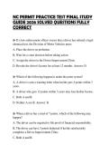
, Probability Current
We can define a
probability current ; (x) as the
probability per time passing through a fixed point so for a
given wave function
NC t). . If j(x + x0) #j(x) then the total probability in do will change with time .
t ve dj(xo t) implying
!
,
The net probability current in or out of a line element is : j(x + do t) , -j(x t) ,
=
dj(o t) ,
that probability is flowing
j(x0 t)
,
j(o + dx t) ,
out of the interval
wo r o
a Conservation of probability implies :
dj o
,
t) =
- No .
t)" da
Xo To + dx
Continuity equation : 0 Tr( t)" ,
= -
Oj( t) ,
The greater the magnitude of the slope of the probability
dx
Ot current at positions the,
greater the temporal change in
probability density at that position .
We can
find an expression for j.
·
Using the product rule on the CHS of the equation : (M *N )
continuity =***
Assuming
-N VN
=
TDSE -
T satisfies the
· :
+ =
Ot Ot
-Vi
* * *
·
The complex conjugate of the TDSE is :
·
Inserting these into the expanded
continuity equation :
=N N
*N)
N
+
Ra
= -N we want to write the o e
-
the
probability current.
We can use the fact that
:* -
*
=
N
2
Thus we obtain N*
: =N
Hence j(t) :
= /
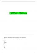
The Infinite Square Well
Solving the TISE for a Particle in a Box
[
for 10
The associated potential energy for a ID
infinite square well of width a : V() =
for 0 = a
D
for x = a
Time Dependent
total energy operator
- T(x ,
t) + VT t) ,
=
it Tr(x t) ,
C FN iM =
TDSE
Im d ↳ -Stax only depends
V =
on c ,
not .
out
-
Kinetic
energy operator Potential energy operator
The momentum operator p -it : =
The Kinetic energy operator F : =
-
The operator representing the total
energy (the Hamiltonian)
H : = + V = -ve
The TDSE is a linear differential equation -
implies that the superposition principle holds : If M and M are solutions,
then AT + BT is also a solution. Thus
given quantum system energy eigen functions (with definite energy
for a ,
as well as superposition states (with simultaneous multiple energies) satisfy the TDSE .
The TDSE time the wave function TG to) at some time to uniquely determines the
is first order in
specifying
-
,
wave function at a later time (if no measurement is taken/the system is unperturbed). Thus the quantum state
evolves deterministically.
Time-Independent
We only consider timeindependent potential energies
-
V(),
so we can write the energy eigenfunction as a
product of a
Spatial and a temporal solution :
↑(x t) u(x) T(t) only the form of not of superposition states
eigenfunctions
=
energy
=
, ,
Inserting this into the TDSE we obtain : - Ub T(t) + Vbc)uk) T(t) =
in ux T(t) (= u() + (t)
Dividing into (C) and (t) terms gives :
- + V
=
Bothsides must be equal to the same constant with units of energy ,
as it must have the same unit as V() -
> E
which denotes the total
energy .
We obtain the TISE
by setting the LHS equal to E and
multiplying by u (x) :
Flu
- u(x) Vu() Enk) or El
=
+ =
The TISE is an
energy eigenvalue equation with energy eigenfunction () and energy eigenvalue E Thus,
, .
only quantum states with definite
energy (zero uncertainty) can solve the TISE (unlike the TDSE which can be
solved by both energy eigenfunctions and superposition states).
We can obtain the temporal solution by the RHS equal to E
setting
-
iEt
and multiplying by Tt)
dT(t) =
-
iET(t) >
-
T(t) = et = temporal solution for any potential energy VGC)
dt h
, Conditions for Quantum Mechanical Wave functions
*
In one dimension the probability density ↑N T N is a probability length with units [m-] . Thus N t)>
per
=
,
is the probability position measurement of the particle in the interval da
,
upon , finding .
·
Normalisation condition : (% 2 dx =
1
Any function f(x) that is square-integrable can be normalised : ( f(x)x = a # f(x) is correctly
A function is
only square-integrable if M t) > 0 as C-10 . normalised
+
,
·
In addition to being normalised ,
a valid wave function must be continuous -
a
discontinuity would lead to
ambigious probabilities .
·
The slope of must also be continuous , except at points where the potential energy is infinite.
uk) Em(Vx-Eu Integrating
= consider the slope of u() at a point e . over the small
interval (x,-E x + E) gives ,
.
:
+ Em(V(x) -
E)u(x)dx
+- = (V(x) -
E)u(x)dx I the LHS * 0 in the limit -o then
& is discontinuous at ..
As Eu(x) is finite the integral
,
will tend to zero as E-> 0 .
Even if VG) is discontinuous at x but finite on either side ,
the integral VG)uGd will tend to zero as 3- 0 .
The RHS #0 only if UGC) is infinite.
If we assume a Dirac delta peaked at , with V6) =
-go(x -
x ,) then we
get :
- u(x-2) -u
du(x , + 2) =
-
da
that there is in the
so a
discontinuity slope at >, if uk) to
The Expectation Value of an Operator
In
general taking a measurement of a property of a quantum particle changes its state we cannot perform
-
,
successive measurements prepare many identical states then perform a measurement on each system .
-
The expectation value of an operator is the average measurement outcome.
for any operator 0 with discrete outcomes (eg energy)
.
: 0 v
=
[0 : Prob(0 ) :
for
any operator ? with continuous outcomes (eg .
position ,
momentum) : v = N* No
Quantum Uncertainty
The Heisenberg uncertainty principle C Do has the following consequences :
with a well-defined wave function does not possess a well-defined
A particle trajectory
·
·
Localisation costs energy all particles confined to-
a finite region of space must possess
Kinetic
energy
·
Classical ideas of causality break down .
Quantum uncertainty : (2) -
(8)2
Mathematically the quantum uncertainty of
,
an observable is the standard deviation of the underlying
probability distribution prior to measurement .
, Probability Current
We can define a
probability current ; (x) as the
probability per time passing through a fixed point so for a
given wave function
NC t). . If j(x + x0) #j(x) then the total probability in do will change with time .
t ve dj(xo t) implying
!
,
The net probability current in or out of a line element is : j(x + do t) , -j(x t) ,
=
dj(o t) ,
that probability is flowing
j(x0 t)
,
j(o + dx t) ,
out of the interval
wo r o
a Conservation of probability implies :
dj o
,
t) =
- No .
t)" da
Xo To + dx
Continuity equation : 0 Tr( t)" ,
= -
Oj( t) ,
The greater the magnitude of the slope of the probability
dx
Ot current at positions the,
greater the temporal change in
probability density at that position .
We can
find an expression for j.
·
Using the product rule on the CHS of the equation : (M *N )
continuity =***
Assuming
-N VN
=
TDSE -
T satisfies the
· :
+ =
Ot Ot
-Vi
* * *
·
The complex conjugate of the TDSE is :
·
Inserting these into the expanded
continuity equation :
=N N
*N)
N
+
Ra
= -N we want to write the o e
-
the
probability current.
We can use the fact that
:* -
*
=
N
2
Thus we obtain N*
: =N
Hence j(t) :
= /
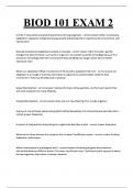
The Infinite Square Well
Solving the TISE for a Particle in a Box
[
for 10
The associated potential energy for a ID
infinite square well of width a : V() =
for 0 = a
D
for x = a