6 Mean-Variance Portfolio Theory
Single investment period: money is invested at the initial time, and payoff is attained at the
end of the period.
Mean-variance analysis
1 Asset return
Asset: an investment instrument that can be bought and sold.
𝑎𝑚𝑜𝑢𝑛𝑡 𝑟𝑒𝑐𝑒𝑖𝑣𝑒𝑑
Total return on your investment: 𝑡𝑜𝑡𝑎𝑙 𝑟𝑒𝑡𝑢𝑟𝑛 = 𝑎𝑚𝑜𝑢𝑛𝑡 𝑖𝑛𝑣𝑒𝑠𝑡𝑒𝑑
- X0 = amount invested
- X1 = amount received
𝑋1
- 𝑅 = 𝑋0
𝑎𝑚𝑜𝑢𝑛𝑡 𝑟𝑒𝑐𝑒𝑖𝑣𝑒𝑑 − 𝑎𝑚𝑜𝑢𝑛𝑡 𝑖𝑛𝑣𝑒𝑠𝑡𝑒𝑑
Rate of return: 𝑟𝑎𝑡𝑒 𝑜𝑓 𝑟𝑒𝑡𝑢𝑟𝑛 = 𝑎𝑚𝑜𝑢𝑛𝑡 𝑖𝑛𝑣𝑒𝑠𝑡𝑒𝑑
𝑋1−𝑋0
- 𝑟 = 𝑋0
- 𝑅=1+𝑟
- 𝑋1 = (1 + 𝑟) 𝑋0
Short selling / shorting: you borrow the asset from someone who owns it and sell it to
someone else, receiving X0. Later, you repurchase the asset for X1 and return it to the lender.
- Profit: X0 - X1
- Risky, potential for loss is unlimited
−𝑋1 𝑋1
- 𝑅 = −𝑋0
= 𝑋0
- − 𝑋1 = − 𝑋0𝑅 = − 𝑋0 (1 + 𝑟)
Master asset / Portfolio: combining different assets.
- 𝑋0𝑖 = 𝑤𝑖 𝑋0
- wi is the weight or fraction of asset i in the portfolio
𝑛
- ∑ 𝑤𝑖 = 1
𝑖=1
- May be negative if short selling is allowed
𝑛
∑ 𝑅𝑖𝑤𝑖𝑋0 𝑛
- Overal return: 𝑅 = 𝑖=1
𝑋0
= ∑ 𝑤𝑖𝑅𝑖
𝑖=1
- Ri = total return of asset i
𝑛
- 𝑟 = ∑ 𝑤𝑖𝑟𝑖
𝑖=1
,Portfolio return: Both the total return and the rate of return of a portfolio of assets are equal
to the weighted sum of the corresponding individual asset returns, with the weight of an
asset being its relative weight (in purchase cost) in the portfolio.
2 Random Variables
The amount of money to be obtained when selling an asset is usually unknown at the time of
purchase, so we see it as a random variable with a probability density function p(x).
𝑚
- 𝐸[𝑥] = ∑ 𝑥𝑖𝑝𝑖
𝑖=1
2
- 𝑣𝑎𝑟(𝑦) = 𝐸[(𝑦 − 𝑦) ]
2 2
- 𝑣𝑎𝑟(𝑥 + 𝑦) = σ𝑥 + 2σ𝑥𝑦 + σ𝑦
- 𝑐𝑜𝑣(𝑥1, 𝑥2) = 𝐸[(𝑥1 − 𝑥1)(𝑥2 − 𝑥2)]
- Covariance bound: The covariance of two random variables satisfies |σ12| ≤ σ1σ2
σ12
- Correlation coefficient: ρ12 = σ1σ2
3 Random Returns
- 𝐸[𝑟] = 𝑟
2 2
- 𝑣𝑎𝑟(𝑟) = 𝐸[(𝑟 − 𝑟) ] = σ
Mean-standard deviation diagram (𝑟 − σ diagram)
4 Portfolio Mean and Variance
Suppose there are n assets with (random) rates of return r1, r2, …, rn.
- 𝐸[𝑟𝑖] = 𝑟𝑖
Rate of return of portfolio:
𝑟 = 𝑤1𝑟1 + 𝑤2𝑟2 + ... + 𝑤𝑛𝑟𝑛
,Mean/Expected return of a portfolio:
𝐸[𝑟] = 𝑤1𝐸[𝑟1] + ... + 𝑤𝑛𝐸[𝑟𝑛]
Variance of portfolio return:
𝑛 𝑛 𝑛 𝑛
2 2 2
σ = 𝐸[(𝑟 − 𝑟) ] = 𝐸[( ∑ 𝑤𝑖𝑟𝑖 − ∑ 𝑤𝑖𝑟𝑖) ] = 𝐸[( ∑ 𝑤𝑖(𝑟𝑖 − 𝑟𝑖))( ∑ 𝑤𝑗(𝑟𝑗 − 𝑟𝑗))]
𝑖=1 𝑖=1 𝑖=1 𝑗=1
𝑛 𝑛
= 𝐸[ ∑ 𝑤𝑖𝑤𝑗(𝑟𝑖 − 𝑟𝑖)(𝑟𝑗 − 𝑟𝑗)] = ∑ 𝑤𝑖𝑤𝑗σ𝑖𝑗
𝑖,𝑗=1 𝑖,𝑗=1
Diversification: the variance of the return of a portfolio can be reduced by including
additional assets in the portfolio.
𝑛
1
If wi = 1/n , the overall rate of return of this portfolio is 𝑟 = 𝑛
∑ 𝑟𝑖
𝑖=1
- Mean value: 𝑟 = 𝑚 (independent from n)
𝑛 2
1 2 σ
- 𝑣𝑎𝑟(𝑟) = 2 ∑ σ = 𝑛
𝑛 𝑖=1
Reducing the variance with diversification usually also reduces the return.
- If the returns are uncorrelated, the variance can be reduced to 0 by taking a large n.
- If the returns are positively correlated, it is more difficult to reduce variance.
Diagram of a Portfolio
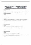
Two assets on a mean-standard deviation diagram can be combined, according to some
weights, to form a portfolio. But since the covariances are not shown on the diagram, the
exact location of the point representing the new asset cannot be determined from the
location on the diagram of the original two assets. There are many possibilities, depending
on the covariance of these asset returns.
- 𝑤1 = 1 − α
- 𝑤2 = α
- α ∈ [0, 1] (or outside of bounds if short selling is allowed)
- As α varies, the new portfolios trace out a curve that includes assets 1 and 2, its
exact curve depends on σ12
Solid portion: positive combinations of the
two assets.
Dashed portion: shorting one of the assets.
Portfolio diagram lemma: The curve in an
𝑟 − σ diagram defined by nonnegative
mixtures of assets 1 and 2 lies within the
triangular region defined by the two original
assets and the point on the vertical axis of
height 𝐴 = (𝑟1σ2 + 𝑟2σ1)/(σ1 + σ2)
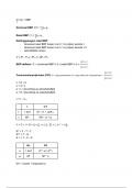
, 5 The Feasible Set
Suppose there are n basic assets, we plot them on the diagram. We find all possible portfolio
combinations of these assets by letting the weighting coefficients wi range over all
𝑛
combinations such that ∑ 𝑤𝑖 = 1. The set of points that corresponds to portfolios is the
𝑖=1
feasible set / feasible region. Two important properties:
1. If there are at least three assets (not perfectly correlated with different means), the
feasible set will be a solid two-dimensional region.
2. The feasible region is convex to the left.
The left boundary of a feasible set is the minimum-variance set, which has a bullet shape.
- Minimum-variance point (MVP)
- Risk averse: chooses a point with the smallest standard deviation for the given
mean.
- Risk preferring: selects a point other than the one of minimum standard deviation.
- Nonsatiation: investors always want more money, they will always pick the portfolio
with the largest mean for a given level of standard deviation.
- Efficient frontier: only the upper part of the minimum-variance set will be of interest
to investors who are risk averse and satisfy nonsatiation.
6 The Markowitz Model
To find a minimum-variance portfolio, we fix the mean value at some arbitrary value 𝑟. Then
we find the feasible portfolio of minimum variance that has this mean.
𝑛 𝑛 𝑛
1
minimize 2
∑ 𝑤𝑖𝑤𝑗σ𝑖𝑗 subject to ∑ 𝑤𝑖𝑟𝑖 = 𝑟 , ∑ 𝑤𝑖 = 1
𝑖,𝑗=1 𝑖=1 𝑖=1
𝑛 𝑛 𝑛
1
Lagrangian: 𝐿 = 2
∑ 𝑤𝑖𝑤𝑗σ𝑖𝑗 − λ ( ∑ 𝑤𝑖𝑟𝑖 − 𝑟) − µ ( ∑ 𝑤𝑖 − 1)
𝑖,𝑗=1 𝑖=1 𝑖=1
- Differentiate with respect to each variable wi and set it to 0.
𝑛
- ∑ σ𝑖𝑗𝑤𝑗 − λ𝑟𝑖 − µ = 0
𝑗=1
Single investment period: money is invested at the initial time, and payoff is attained at the
end of the period.
Mean-variance analysis
1 Asset return
Asset: an investment instrument that can be bought and sold.
𝑎𝑚𝑜𝑢𝑛𝑡 𝑟𝑒𝑐𝑒𝑖𝑣𝑒𝑑
Total return on your investment: 𝑡𝑜𝑡𝑎𝑙 𝑟𝑒𝑡𝑢𝑟𝑛 = 𝑎𝑚𝑜𝑢𝑛𝑡 𝑖𝑛𝑣𝑒𝑠𝑡𝑒𝑑
- X0 = amount invested
- X1 = amount received
𝑋1
- 𝑅 = 𝑋0
𝑎𝑚𝑜𝑢𝑛𝑡 𝑟𝑒𝑐𝑒𝑖𝑣𝑒𝑑 − 𝑎𝑚𝑜𝑢𝑛𝑡 𝑖𝑛𝑣𝑒𝑠𝑡𝑒𝑑
Rate of return: 𝑟𝑎𝑡𝑒 𝑜𝑓 𝑟𝑒𝑡𝑢𝑟𝑛 = 𝑎𝑚𝑜𝑢𝑛𝑡 𝑖𝑛𝑣𝑒𝑠𝑡𝑒𝑑
𝑋1−𝑋0
- 𝑟 = 𝑋0
- 𝑅=1+𝑟
- 𝑋1 = (1 + 𝑟) 𝑋0
Short selling / shorting: you borrow the asset from someone who owns it and sell it to
someone else, receiving X0. Later, you repurchase the asset for X1 and return it to the lender.
- Profit: X0 - X1
- Risky, potential for loss is unlimited
−𝑋1 𝑋1
- 𝑅 = −𝑋0
= 𝑋0
- − 𝑋1 = − 𝑋0𝑅 = − 𝑋0 (1 + 𝑟)
Master asset / Portfolio: combining different assets.
- 𝑋0𝑖 = 𝑤𝑖 𝑋0
- wi is the weight or fraction of asset i in the portfolio
𝑛
- ∑ 𝑤𝑖 = 1
𝑖=1
- May be negative if short selling is allowed
𝑛
∑ 𝑅𝑖𝑤𝑖𝑋0 𝑛
- Overal return: 𝑅 = 𝑖=1
𝑋0
= ∑ 𝑤𝑖𝑅𝑖
𝑖=1
- Ri = total return of asset i
𝑛
- 𝑟 = ∑ 𝑤𝑖𝑟𝑖
𝑖=1
,Portfolio return: Both the total return and the rate of return of a portfolio of assets are equal
to the weighted sum of the corresponding individual asset returns, with the weight of an
asset being its relative weight (in purchase cost) in the portfolio.
2 Random Variables
The amount of money to be obtained when selling an asset is usually unknown at the time of
purchase, so we see it as a random variable with a probability density function p(x).
𝑚
- 𝐸[𝑥] = ∑ 𝑥𝑖𝑝𝑖
𝑖=1
2
- 𝑣𝑎𝑟(𝑦) = 𝐸[(𝑦 − 𝑦) ]
2 2
- 𝑣𝑎𝑟(𝑥 + 𝑦) = σ𝑥 + 2σ𝑥𝑦 + σ𝑦
- 𝑐𝑜𝑣(𝑥1, 𝑥2) = 𝐸[(𝑥1 − 𝑥1)(𝑥2 − 𝑥2)]
- Covariance bound: The covariance of two random variables satisfies |σ12| ≤ σ1σ2
σ12
- Correlation coefficient: ρ12 = σ1σ2
3 Random Returns
- 𝐸[𝑟] = 𝑟
2 2
- 𝑣𝑎𝑟(𝑟) = 𝐸[(𝑟 − 𝑟) ] = σ
Mean-standard deviation diagram (𝑟 − σ diagram)
4 Portfolio Mean and Variance
Suppose there are n assets with (random) rates of return r1, r2, …, rn.
- 𝐸[𝑟𝑖] = 𝑟𝑖
Rate of return of portfolio:
𝑟 = 𝑤1𝑟1 + 𝑤2𝑟2 + ... + 𝑤𝑛𝑟𝑛
,Mean/Expected return of a portfolio:
𝐸[𝑟] = 𝑤1𝐸[𝑟1] + ... + 𝑤𝑛𝐸[𝑟𝑛]
Variance of portfolio return:
𝑛 𝑛 𝑛 𝑛
2 2 2
σ = 𝐸[(𝑟 − 𝑟) ] = 𝐸[( ∑ 𝑤𝑖𝑟𝑖 − ∑ 𝑤𝑖𝑟𝑖) ] = 𝐸[( ∑ 𝑤𝑖(𝑟𝑖 − 𝑟𝑖))( ∑ 𝑤𝑗(𝑟𝑗 − 𝑟𝑗))]
𝑖=1 𝑖=1 𝑖=1 𝑗=1
𝑛 𝑛
= 𝐸[ ∑ 𝑤𝑖𝑤𝑗(𝑟𝑖 − 𝑟𝑖)(𝑟𝑗 − 𝑟𝑗)] = ∑ 𝑤𝑖𝑤𝑗σ𝑖𝑗
𝑖,𝑗=1 𝑖,𝑗=1
Diversification: the variance of the return of a portfolio can be reduced by including
additional assets in the portfolio.
𝑛
1
If wi = 1/n , the overall rate of return of this portfolio is 𝑟 = 𝑛
∑ 𝑟𝑖
𝑖=1
- Mean value: 𝑟 = 𝑚 (independent from n)
𝑛 2
1 2 σ
- 𝑣𝑎𝑟(𝑟) = 2 ∑ σ = 𝑛
𝑛 𝑖=1
Reducing the variance with diversification usually also reduces the return.
- If the returns are uncorrelated, the variance can be reduced to 0 by taking a large n.
- If the returns are positively correlated, it is more difficult to reduce variance.
Diagram of a Portfolio
Two assets on a mean-standard deviation diagram can be combined, according to some
weights, to form a portfolio. But since the covariances are not shown on the diagram, the
exact location of the point representing the new asset cannot be determined from the
location on the diagram of the original two assets. There are many possibilities, depending
on the covariance of these asset returns.
- 𝑤1 = 1 − α
- 𝑤2 = α
- α ∈ [0, 1] (or outside of bounds if short selling is allowed)
- As α varies, the new portfolios trace out a curve that includes assets 1 and 2, its
exact curve depends on σ12
Solid portion: positive combinations of the
two assets.
Dashed portion: shorting one of the assets.
Portfolio diagram lemma: The curve in an
𝑟 − σ diagram defined by nonnegative
mixtures of assets 1 and 2 lies within the
triangular region defined by the two original
assets and the point on the vertical axis of
height 𝐴 = (𝑟1σ2 + 𝑟2σ1)/(σ1 + σ2)
, 5 The Feasible Set
Suppose there are n basic assets, we plot them on the diagram. We find all possible portfolio
combinations of these assets by letting the weighting coefficients wi range over all
𝑛
combinations such that ∑ 𝑤𝑖 = 1. The set of points that corresponds to portfolios is the
𝑖=1
feasible set / feasible region. Two important properties:
1. If there are at least three assets (not perfectly correlated with different means), the
feasible set will be a solid two-dimensional region.
2. The feasible region is convex to the left.
The left boundary of a feasible set is the minimum-variance set, which has a bullet shape.
- Minimum-variance point (MVP)
- Risk averse: chooses a point with the smallest standard deviation for the given
mean.
- Risk preferring: selects a point other than the one of minimum standard deviation.
- Nonsatiation: investors always want more money, they will always pick the portfolio
with the largest mean for a given level of standard deviation.
- Efficient frontier: only the upper part of the minimum-variance set will be of interest
to investors who are risk averse and satisfy nonsatiation.
6 The Markowitz Model
To find a minimum-variance portfolio, we fix the mean value at some arbitrary value 𝑟. Then
we find the feasible portfolio of minimum variance that has this mean.
𝑛 𝑛 𝑛
1
minimize 2
∑ 𝑤𝑖𝑤𝑗σ𝑖𝑗 subject to ∑ 𝑤𝑖𝑟𝑖 = 𝑟 , ∑ 𝑤𝑖 = 1
𝑖,𝑗=1 𝑖=1 𝑖=1
𝑛 𝑛 𝑛
1
Lagrangian: 𝐿 = 2
∑ 𝑤𝑖𝑤𝑗σ𝑖𝑗 − λ ( ∑ 𝑤𝑖𝑟𝑖 − 𝑟) − µ ( ∑ 𝑤𝑖 − 1)
𝑖,𝑗=1 𝑖=1 𝑖=1
- Differentiate with respect to each variable wi and set it to 0.
𝑛
- ∑ σ𝑖𝑗𝑤𝑗 − λ𝑟𝑖 − µ = 0
𝑗=1