Statistics DSS (25spring)
Notes & Study Guide
Number in tle refers to corresponding Module
(order of module is adjusted for clearer structure)
With sign: given quiz & exam sample ques ons
To pass or get a good score in final exam, it is strongly
recommended to thoroughly engage with the material
and gain a deep understanding of the concepts and
terms.
Any ques on, please email to:
Version: 202503201719
By: Alice
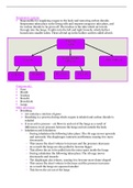
, Statistical reasoning(1)
Sta s cal reasoning the founda on of all good sta s cal analyses is a deliberate careful, and thorough
considera on of uncertainty.
The purpose of sta s cs to systema ze the way that we account for uncertainty when making data-based
decisions
No need to memorize any formulas the larger the test sta s cs, the be er. (In general)
unless teacher specifically says so
(Week 1 Basic 3, 02:51) (Sta s cs is all about what we can see as human and how we decide based on what we see,
it is not about how the real world actually is)
Probability distribu on quan fy how likely it is to observe each possible value of some probabilis c en ty
(re-scaled frequency distribu ons) (e.g. height, the outcome variable)
Sta s cal Tes ng dis ll info into a simple sta s c to make a judgement, we weight the es mated effect
by the precision of the es mate.
Wald Test 𝑇=
Nil-null a null hypothesis of no effect Very Important: the possible value of test sta s c
t-test a way to summarize the comparison of two variables’ distribu on
the t-sta s c also has a sampling distribu on that quan fies the possible t-values we
could get if we repeatedly drew samples from the variables’ distribu on and re-
computed a t-sta s c each me.
Direc onal hypothesis
NOT a test sta s c P value
𝑃(𝑡 = 𝑡̂|𝐻 ) = 0 (the probability of observing any individual point on a con nuous
(Week 1 Part 1 Quiz 2) distribu on is exactly zero.)
CAN NOT say There is a 0.032 probability that the true mean difference is greater than zero.
There is a 0.032 probability that the null hypothesis is false.
There is a 0.032 probability that the observed result is due to chance alone.
There is a 0.032 probability of replica ng the observed effect in the future.
There is a 0.032 probability of observing 𝑡̂, if the null hypothesis is true.
How do we interpret the p value then? There is a 0.032 probability of observing a test sta s c at least as large as 𝒕, if the null
hypothesis is true. 𝑃(𝑡 ≥ 𝑡̂|𝐻 )
What do we want to know? The inversed ques on: what is the probability of the null hypothesis is true, given that
*not possible with null-hypothesis tes ng a t-sta s c is larger or equal than the es mated one?
possible only with Bayesian sta s cs
In what scenario do we use in experimental contexts.
sta s cal tes ng? While real world has messy observa onal data, has no control for confounding factors.
We need sta s cal modeling.
Sta s cal modeling build a mathema cal representa on of the (interes ng aspects) of a data distribu on
-> learn the important features of a distribu on (without a prior hypothesis)
Data Science Cycle (4 essen al steps) define a problem – collect data – process data – clean data (slide week 1 design p4)
Collec ng own data is NOT always preferred over secondary data (week 1 part 2 quiz 2)
EDA (Exploratory data analysis) 1) mindset than techniques/steps; 2) contrast with strict empiricist hypothesis tes ng
3) be used to generate hypotheses for CDA; 4) sanity check hypotheses, if fail, reject.
(can’t modify hypotheses based on these sanity checks and s ll test new hypotheses with the same data)
5) if don’t care about tes ng hypotheses, focus on EDA.
CDA (confirmatory data analysis) 1) if data are well-understood, proceed directly to CDA;
*CDA and EDA can NOT stand alone
, Outliers(2)
What is univariate outlier? Extreme values with respect to the distribu on of a variable’s other observa ons
- illegal value: data entry errors (most common cause)
- legal value: extreme values (e.g. a person 3-meter high)
We choose to view an outlier as arising from a different popula on than the one to
which we want to generalize our findings.
What are the methods to diagnose
poten al outliers?
1.Internally studen zed residuals for each observa on 𝑋 : 𝑇 =
(Z-score method)
𝑇 follows a student’s t distribu on with df = N – 1
This means any point that is not an outlier we can do a formal test for “outlier” status, assuming a large sample
should not be too far from mean if 𝑇 > 𝐶 (C is usually 2 or 3), we label 𝑋 as an outlier
we define how far it is in terms of SD Cons:
- C (cut-point) can only be meaningfully chosen when X is normally distributed
- Both 𝑋 and 𝑆𝐷 are highly sensi ve to outliers
2.Externally studen zed residuals internally studen zed residuals but adjust 𝑋 and 𝑆𝐷 to remove the influence of
outlier itself will affect mean and sd observa on we are evalua ng. dele on mean, dele on SD
Pros:
T(n) is immune the influence of the n-th observa on.
Cons:
- X is s ll required to be normally distributed
- can s ll be sensi ve to other outlier that is not n-th oberva on
3. Median absolute devia on method mean of X -> Med of X, SD -> median absolute devia on (MAD)
𝑀𝐴𝐷 = 𝑏 ∗ 𝑀𝑒𝑑(|𝑋 − 𝑀𝑒𝑑(𝑋)|) Pros: Immune to the influence of (50% at most) outliers.
𝑏=1 𝑄 = 1 0.6745 Cons:
.
(normal distribu on) - does not allow for formal sta s cal tests
- X is required to be parametric distribu on (need to compute b)
4. Tukey’s boxplot method Pros: does not require normally distributed X, not sensi ve to outliers
𝐼𝑄𝑅 = 𝑄 − 𝑄 Cons: does not allow for formal sta s cal tests
𝐹 = {𝑄 − 𝐶 ∗ 𝐼𝑄𝑅, 𝑄 + 𝐶 ∗ 𝐼𝑄𝑅}
C Fence Type Outlier Type Mean Dele on Mean Median Boxplot Method
1.5 Inner Possible 1/N 2/N N/2 25%
3 Outer Probable
Breakdown Point the minimum propor on of cased that must be replaced by inf to cause
the value of sta s c to go to inf
Mul variate Outliers e.g. a person in the 95th percen le for height & the 5th percen le for weight
How do we detect it?
Distance metrics quan fy the similarity of two vectors (similarity between an observa on & mean vector)
- Mahalanobis distance mul variate generaliza on of internally studen zed residual
Cons: it is compute using all observa ons, so sensi ve to outlier also.
- Robust Mahalanobis distance Minimum covariance determinant method(MCD), using only good subset of data to es mate
How far away an observa on is from the center of data cloud, rela ve to the size of cloud
Use less observa on of data therefore less influenced by outliers
Notes & Study Guide
Number in tle refers to corresponding Module
(order of module is adjusted for clearer structure)
With sign: given quiz & exam sample ques ons
To pass or get a good score in final exam, it is strongly
recommended to thoroughly engage with the material
and gain a deep understanding of the concepts and
terms.
Any ques on, please email to:
Version: 202503201719
By: Alice
, Statistical reasoning(1)
Sta s cal reasoning the founda on of all good sta s cal analyses is a deliberate careful, and thorough
considera on of uncertainty.
The purpose of sta s cs to systema ze the way that we account for uncertainty when making data-based
decisions
No need to memorize any formulas the larger the test sta s cs, the be er. (In general)
unless teacher specifically says so
(Week 1 Basic 3, 02:51) (Sta s cs is all about what we can see as human and how we decide based on what we see,
it is not about how the real world actually is)
Probability distribu on quan fy how likely it is to observe each possible value of some probabilis c en ty
(re-scaled frequency distribu ons) (e.g. height, the outcome variable)
Sta s cal Tes ng dis ll info into a simple sta s c to make a judgement, we weight the es mated effect
by the precision of the es mate.
Wald Test 𝑇=
Nil-null a null hypothesis of no effect Very Important: the possible value of test sta s c
t-test a way to summarize the comparison of two variables’ distribu on
the t-sta s c also has a sampling distribu on that quan fies the possible t-values we
could get if we repeatedly drew samples from the variables’ distribu on and re-
computed a t-sta s c each me.
Direc onal hypothesis
NOT a test sta s c P value
𝑃(𝑡 = 𝑡̂|𝐻 ) = 0 (the probability of observing any individual point on a con nuous
(Week 1 Part 1 Quiz 2) distribu on is exactly zero.)
CAN NOT say There is a 0.032 probability that the true mean difference is greater than zero.
There is a 0.032 probability that the null hypothesis is false.
There is a 0.032 probability that the observed result is due to chance alone.
There is a 0.032 probability of replica ng the observed effect in the future.
There is a 0.032 probability of observing 𝑡̂, if the null hypothesis is true.
How do we interpret the p value then? There is a 0.032 probability of observing a test sta s c at least as large as 𝒕, if the null
hypothesis is true. 𝑃(𝑡 ≥ 𝑡̂|𝐻 )
What do we want to know? The inversed ques on: what is the probability of the null hypothesis is true, given that
*not possible with null-hypothesis tes ng a t-sta s c is larger or equal than the es mated one?
possible only with Bayesian sta s cs
In what scenario do we use in experimental contexts.
sta s cal tes ng? While real world has messy observa onal data, has no control for confounding factors.
We need sta s cal modeling.
Sta s cal modeling build a mathema cal representa on of the (interes ng aspects) of a data distribu on
-> learn the important features of a distribu on (without a prior hypothesis)
Data Science Cycle (4 essen al steps) define a problem – collect data – process data – clean data (slide week 1 design p4)
Collec ng own data is NOT always preferred over secondary data (week 1 part 2 quiz 2)
EDA (Exploratory data analysis) 1) mindset than techniques/steps; 2) contrast with strict empiricist hypothesis tes ng
3) be used to generate hypotheses for CDA; 4) sanity check hypotheses, if fail, reject.
(can’t modify hypotheses based on these sanity checks and s ll test new hypotheses with the same data)
5) if don’t care about tes ng hypotheses, focus on EDA.
CDA (confirmatory data analysis) 1) if data are well-understood, proceed directly to CDA;
*CDA and EDA can NOT stand alone
, Outliers(2)
What is univariate outlier? Extreme values with respect to the distribu on of a variable’s other observa ons
- illegal value: data entry errors (most common cause)
- legal value: extreme values (e.g. a person 3-meter high)
We choose to view an outlier as arising from a different popula on than the one to
which we want to generalize our findings.
What are the methods to diagnose
poten al outliers?
1.Internally studen zed residuals for each observa on 𝑋 : 𝑇 =
(Z-score method)
𝑇 follows a student’s t distribu on with df = N – 1
This means any point that is not an outlier we can do a formal test for “outlier” status, assuming a large sample
should not be too far from mean if 𝑇 > 𝐶 (C is usually 2 or 3), we label 𝑋 as an outlier
we define how far it is in terms of SD Cons:
- C (cut-point) can only be meaningfully chosen when X is normally distributed
- Both 𝑋 and 𝑆𝐷 are highly sensi ve to outliers
2.Externally studen zed residuals internally studen zed residuals but adjust 𝑋 and 𝑆𝐷 to remove the influence of
outlier itself will affect mean and sd observa on we are evalua ng. dele on mean, dele on SD
Pros:
T(n) is immune the influence of the n-th observa on.
Cons:
- X is s ll required to be normally distributed
- can s ll be sensi ve to other outlier that is not n-th oberva on
3. Median absolute devia on method mean of X -> Med of X, SD -> median absolute devia on (MAD)
𝑀𝐴𝐷 = 𝑏 ∗ 𝑀𝑒𝑑(|𝑋 − 𝑀𝑒𝑑(𝑋)|) Pros: Immune to the influence of (50% at most) outliers.
𝑏=1 𝑄 = 1 0.6745 Cons:
.
(normal distribu on) - does not allow for formal sta s cal tests
- X is required to be parametric distribu on (need to compute b)
4. Tukey’s boxplot method Pros: does not require normally distributed X, not sensi ve to outliers
𝐼𝑄𝑅 = 𝑄 − 𝑄 Cons: does not allow for formal sta s cal tests
𝐹 = {𝑄 − 𝐶 ∗ 𝐼𝑄𝑅, 𝑄 + 𝐶 ∗ 𝐼𝑄𝑅}
C Fence Type Outlier Type Mean Dele on Mean Median Boxplot Method
1.5 Inner Possible 1/N 2/N N/2 25%
3 Outer Probable
Breakdown Point the minimum propor on of cased that must be replaced by inf to cause
the value of sta s c to go to inf
Mul variate Outliers e.g. a person in the 95th percen le for height & the 5th percen le for weight
How do we detect it?
Distance metrics quan fy the similarity of two vectors (similarity between an observa on & mean vector)
- Mahalanobis distance mul variate generaliza on of internally studen zed residual
Cons: it is compute using all observa ons, so sensi ve to outlier also.
- Robust Mahalanobis distance Minimum covariance determinant method(MCD), using only good subset of data to es mate
How far away an observa on is from the center of data cloud, rela ve to the size of cloud
Use less observa on of data therefore less influenced by outliers