Statistics I
STAT
Grade
Three assignments of the workgroups accounting for 20%
Participation accounting for 10%
Exam – 70%
Open and closed questions
Minimum grade of five
Lectures – week 1
Variables and levels of measurement
Variable – any characteristics, number, or quantity that can be measured
and can differ across entities or across time
Variables have different scales or levels of measurement
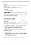
Levels of measurement – nature of
information of the values assigned to
variables
Types of levels
Nominal variable – type of categorical
variable that includes two or more
exclusive categories with no natural order
Ordinal variable – type of categorical variable with clear ordering of the
values
E.g. low <-> high, little <-> much, small <-> large
Distance between values not the same across the levels
Relative comparison
Numerical variable – a variable where the measurement is typically
represented by numbers
Continuous variable – a continuous numeric variable can be measured to
any level of precision
Alternative levels of measurement - two forms of continuous variables
(Stanley smith Stevens);
- Interval – numerical variable but the zero is arbitrary/meaningless
- Ratio – like interval but meaningful zero
Discrete variables – cannot be measured to any level of precision, only
certain, countable values (usually whole numbers) are possible
,Explanatory & response variables
Explanatory (independent) variable
Cause
Often written as X
Response (dependent) variable
Outcome
Often written as Y
Organizing variables
Common format of dataset
- Each column = particular variable
- Each row = given record of the data set in question
- Each cell = one observation on one element in our dataset
Measures of central tendency
Distribution
When we collect data, we can show how the values are distributed in
relation to other values
Frequency distribution – display of the pattern of frequencies of a variable
of a data set
Show all the possible values (or intervals) of the data and how often
they occur
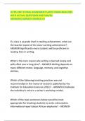
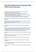
Skewness and symmetry
There is an infinite number of distributions – symmetrical, bimodal,
multimodal
Asymmetrical distributions
Negative (left) skew – mass concentrated on the right; left tail is longer
Positive (right) skew – mass concentrated on the left; right tail is longer
How can we summarise/describe distributions of variables
Option 1 – visualize data
Option 2 – calculate measures to summarise data
, Measure of central tendency – a value that describes a set of data by
identifying the central position within that set of data
Measure of dispersion – how stretched or squeezed is the distribution
Level of measurement Measures of central tendency
Nominal Mode
Ordinal Median + mode
Numeric Mean + median + mode
Mode – the most frequent score in a data set
There can be several modes
Median – middle score for a set of data that has been arranged in order of
magnitude
Even number of scores -> convention add two numbers in the middle
and divide them by two
(Arithmetic) Mean:
Mean is sensitive to extreme values (outliers)
- If extreme values are in the data set the median may be more useful
Median – robust statistic
Measures of dispersion
How stretched or squeezed is the distribution
Level of measurement Measure of dispersion
Nominal No measure of dispersion possible
Ordinal Range, inter-quartile range
Numeric Range, inter-quartile range,
variance/standard deviation
The range – the difference between the lowest and highest value
Range = maximum – minimum
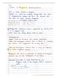
Range & interquartile range
We can split data into chunks (quantiles)
Many quantiles exist but some are common;
Percentile; distribution is divided into 100 parts
Deciles; distribution is divided into 1o parts
Quintiles; distribution is divided into 5 parts
Quartiles; distribution is divided into 3 parts
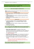
A common form of range – interquartile range
The IQR is the range of the middle 50% of the data
, Calculated by subtracting the 1st quartile from the 3rd quartile
- First quartile Q1 – median of the 50% smallest entries
- Third quartile Q3 – median of the 50% largest entries
Variance and standard deviation
Problem – interquartile range uses only a selection of data (which makes it
robust against outliers)
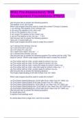
Measures of spread using all data – deviance = Xi – X (difference between
value and mean)
Once we have the deviance of all we can calculate the sum of all
deviances: total deviance ->
Total deviance:
Problem – total deviance is always zero (negative and positive deviations)
Not a useful measure of spread
Instead we calculate the sum of squared errors (SS) ->
Two steps
1) Square the deviances (difference between mean and values)
2) Add the squared deviances
Variances (s2)
Problem – increase of n (number of observations) – increase of sum of
squared errors
- Not a useful measure to compare
Solution – divide sum of squared errors by number of observations (N)
minus 1
*n – 1 is bessels correction
Standard deviation (s)
Larger standard deviation – bigger spread/dispersion around the mean
The standard deviation is dependent on the scale
STAT
Grade
Three assignments of the workgroups accounting for 20%
Participation accounting for 10%
Exam – 70%
Open and closed questions
Minimum grade of five
Lectures – week 1
Variables and levels of measurement
Variable – any characteristics, number, or quantity that can be measured
and can differ across entities or across time
Variables have different scales or levels of measurement
Levels of measurement – nature of
information of the values assigned to
variables
Types of levels
Nominal variable – type of categorical
variable that includes two or more
exclusive categories with no natural order
Ordinal variable – type of categorical variable with clear ordering of the
values
E.g. low <-> high, little <-> much, small <-> large
Distance between values not the same across the levels
Relative comparison
Numerical variable – a variable where the measurement is typically
represented by numbers
Continuous variable – a continuous numeric variable can be measured to
any level of precision
Alternative levels of measurement - two forms of continuous variables
(Stanley smith Stevens);
- Interval – numerical variable but the zero is arbitrary/meaningless
- Ratio – like interval but meaningful zero
Discrete variables – cannot be measured to any level of precision, only
certain, countable values (usually whole numbers) are possible
,Explanatory & response variables
Explanatory (independent) variable
Cause
Often written as X
Response (dependent) variable
Outcome
Often written as Y
Organizing variables
Common format of dataset
- Each column = particular variable
- Each row = given record of the data set in question
- Each cell = one observation on one element in our dataset
Measures of central tendency
Distribution
When we collect data, we can show how the values are distributed in
relation to other values
Frequency distribution – display of the pattern of frequencies of a variable
of a data set
Show all the possible values (or intervals) of the data and how often
they occur
Skewness and symmetry
There is an infinite number of distributions – symmetrical, bimodal,
multimodal
Asymmetrical distributions
Negative (left) skew – mass concentrated on the right; left tail is longer
Positive (right) skew – mass concentrated on the left; right tail is longer
How can we summarise/describe distributions of variables
Option 1 – visualize data
Option 2 – calculate measures to summarise data
, Measure of central tendency – a value that describes a set of data by
identifying the central position within that set of data
Measure of dispersion – how stretched or squeezed is the distribution
Level of measurement Measures of central tendency
Nominal Mode
Ordinal Median + mode
Numeric Mean + median + mode
Mode – the most frequent score in a data set
There can be several modes
Median – middle score for a set of data that has been arranged in order of
magnitude
Even number of scores -> convention add two numbers in the middle
and divide them by two
(Arithmetic) Mean:
Mean is sensitive to extreme values (outliers)
- If extreme values are in the data set the median may be more useful
Median – robust statistic
Measures of dispersion
How stretched or squeezed is the distribution
Level of measurement Measure of dispersion
Nominal No measure of dispersion possible
Ordinal Range, inter-quartile range
Numeric Range, inter-quartile range,
variance/standard deviation
The range – the difference between the lowest and highest value
Range = maximum – minimum
Range & interquartile range
We can split data into chunks (quantiles)
Many quantiles exist but some are common;
Percentile; distribution is divided into 100 parts
Deciles; distribution is divided into 1o parts
Quintiles; distribution is divided into 5 parts
Quartiles; distribution is divided into 3 parts
A common form of range – interquartile range
The IQR is the range of the middle 50% of the data
, Calculated by subtracting the 1st quartile from the 3rd quartile
- First quartile Q1 – median of the 50% smallest entries
- Third quartile Q3 – median of the 50% largest entries
Variance and standard deviation
Problem – interquartile range uses only a selection of data (which makes it
robust against outliers)
Measures of spread using all data – deviance = Xi – X (difference between
value and mean)
Once we have the deviance of all we can calculate the sum of all
deviances: total deviance ->
Total deviance:
Problem – total deviance is always zero (negative and positive deviations)
Not a useful measure of spread
Instead we calculate the sum of squared errors (SS) ->
Two steps
1) Square the deviances (difference between mean and values)
2) Add the squared deviances
Variances (s2)
Problem – increase of n (number of observations) – increase of sum of
squared errors
- Not a useful measure to compare
Solution – divide sum of squared errors by number of observations (N)
minus 1
*n – 1 is bessels correction
Standard deviation (s)
Larger standard deviation – bigger spread/dispersion around the mean
The standard deviation is dependent on the scale