ECB2METRIE – Econometrics
Utrecht University School of Economics
2023-2024 Academic Season
, Econometrics
Week 1: Overview of regression analysis and basic
properties/assumptions of OLS
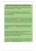
Regression Analysis: Terminology
Population: purely theoretical
Sample: empirical counterpart
Where:
- Y: dependent variable (explained/endogenous/regressand)
- X1: independent variable (explanatory/exogenous/regressors)
o If multiple independent variables (X2 … Xk) = multivariate regression
- ε: error term (disturbance) – captures all other influences on Y (other than the influences of the
independent variables)
o is the error term uncorrelated with the error term – exogenous
o is the error term correlated with the error term - endogenous
Using the regression formulae, we can
- Estimation = using equation for sample using the OLS estimator.
- Inference = use the sample equation to say something about the population equation, by using the
sampling distribution of B̂k
Terminology of the multiple regression model:
Population regression model takes the general form:
Where;
- Yi = dependent variable
- X1, X2, … Xk are independent variables
- E = error term
What is the multiple regression model?
- Regression of Y on X
- Models the effect of the X’s (independent variables) on the Y
, Econometrics
- The regression equation is linear in parameters B0, B1, B2 … Bk
- Subscript i indexes individual population observations (1 through N)
In general form:
Where;
- B0, B1, B2 … Bk are the population parameters (coefficients)
- B0: intercept/constant – expected value of Y when X1 = X2 = … Xk = 0
- B1, B2 … Bk: slope parameters
- B1: expected effect of a one-unit change in X1 on Y; holding X2, X3 … Xk constant
Question: When can B1 be interpreted as a causal effect on X1 on Y, ceteris paribus? Following example
shows this, when the expectation of the value of the error term is equal to zero.
Example model to demonstrate causality in the multiple regression model
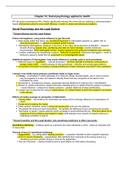
This model informs us about how starting wages (W) relate to the gender (G) and age (A) of graduates. We
can then write the expected wage for a female (binary variable where M=0, F=1) graduate aged 25 as:
We can calculate the expectation value:
Expected wage for 25-year old graduate female:
Same goes for a 26-year old graduate female, as below:
, Econometrics
With the difference between the two being the causal impact of being one-year older on wages, ceteris
paribus, on gender – this is given by B2, if and only if E[e|(G,A)] = 0:
In general, causality in the multiple regression model, is a conditional mean assumption. Under this
assumption, we can interpret our estimates as causal.
Bivariate regression analysis
We turn back to:
Population: purely theoretical
Sample: empirical counterpart
In bivariate regression analysis, we analyse two variables to establish the strength of the relationship
between them (X (ind.) and Y(dep.))
Some facts: Looking back in economics, one of the most pressing themes in economic study is inequality.
Since the 1980s, income inequality in advanced countries has seemed to increase. Part of this sharp
increase that has garnered a lot of attention is the rapid rise of incomes at the very top of the distribution.
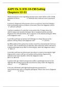
Some of this can be accounted for by skyrocketing pay for CEOs. We can perform a bivariate regression
analysis on CEO pay:
RQ: Is CEO pay in 1999 linked to 1998 profits?
- Payi : salary + bonuses of the CEO of the ith company
- Profiti : the profit of the ith company
Economic theory to support HA
- Rewards for creating shareholder value
- Performance pay (give CEO incentive to increase company profits)
We use a sample of Fortune500 companies, containing the following information:
- CEO pay in 1999 measured in $thousands
- Profits of 1998 in $millions.
Sample regression model:
Utrecht University School of Economics
2023-2024 Academic Season
, Econometrics
Week 1: Overview of regression analysis and basic
properties/assumptions of OLS
Regression Analysis: Terminology
Population: purely theoretical
Sample: empirical counterpart
Where:
- Y: dependent variable (explained/endogenous/regressand)
- X1: independent variable (explanatory/exogenous/regressors)
o If multiple independent variables (X2 … Xk) = multivariate regression
- ε: error term (disturbance) – captures all other influences on Y (other than the influences of the
independent variables)
o is the error term uncorrelated with the error term – exogenous
o is the error term correlated with the error term - endogenous
Using the regression formulae, we can
- Estimation = using equation for sample using the OLS estimator.
- Inference = use the sample equation to say something about the population equation, by using the
sampling distribution of B̂k
Terminology of the multiple regression model:
Population regression model takes the general form:
Where;
- Yi = dependent variable
- X1, X2, … Xk are independent variables
- E = error term
What is the multiple regression model?
- Regression of Y on X
- Models the effect of the X’s (independent variables) on the Y
, Econometrics
- The regression equation is linear in parameters B0, B1, B2 … Bk
- Subscript i indexes individual population observations (1 through N)
In general form:
Where;
- B0, B1, B2 … Bk are the population parameters (coefficients)
- B0: intercept/constant – expected value of Y when X1 = X2 = … Xk = 0
- B1, B2 … Bk: slope parameters
- B1: expected effect of a one-unit change in X1 on Y; holding X2, X3 … Xk constant
Question: When can B1 be interpreted as a causal effect on X1 on Y, ceteris paribus? Following example
shows this, when the expectation of the value of the error term is equal to zero.
Example model to demonstrate causality in the multiple regression model
This model informs us about how starting wages (W) relate to the gender (G) and age (A) of graduates. We
can then write the expected wage for a female (binary variable where M=0, F=1) graduate aged 25 as:
We can calculate the expectation value:
Expected wage for 25-year old graduate female:
Same goes for a 26-year old graduate female, as below:
, Econometrics
With the difference between the two being the causal impact of being one-year older on wages, ceteris
paribus, on gender – this is given by B2, if and only if E[e|(G,A)] = 0:
In general, causality in the multiple regression model, is a conditional mean assumption. Under this
assumption, we can interpret our estimates as causal.
Bivariate regression analysis
We turn back to:
Population: purely theoretical
Sample: empirical counterpart
In bivariate regression analysis, we analyse two variables to establish the strength of the relationship
between them (X (ind.) and Y(dep.))
Some facts: Looking back in economics, one of the most pressing themes in economic study is inequality.
Since the 1980s, income inequality in advanced countries has seemed to increase. Part of this sharp
increase that has garnered a lot of attention is the rapid rise of incomes at the very top of the distribution.
Some of this can be accounted for by skyrocketing pay for CEOs. We can perform a bivariate regression
analysis on CEO pay:
RQ: Is CEO pay in 1999 linked to 1998 profits?
- Payi : salary + bonuses of the CEO of the ith company
- Profiti : the profit of the ith company
Economic theory to support HA
- Rewards for creating shareholder value
- Performance pay (give CEO incentive to increase company profits)
We use a sample of Fortune500 companies, containing the following information:
- CEO pay in 1999 measured in $thousands
- Profits of 1998 in $millions.
Sample regression model: