Chapter 7 Power Relations and Circuit Measurements
7.1 Instantaneous and Average Power
Resistor
If a voltage v = Vmcos(t + ) is i
p
applied to a resistor R (Figure
7.1.1a), the current through the + t
v R
– - i
resistor is i = I m cos (ωt+θ) , where v
Vm (a) (b)
I m= Figure 7.1.1
R , and the instantaneous
power dissipated in the resistor at any time t is:
VmIm
=
2
[ 1+cos 2 ( ωt +θ ) ]
p = vi = VmImcos2(t + ) (7.1.1)
The instantaneous power varies at twice the supply frequency and is never negative,
since the resistor does not return power to the supply (Figure 7.1.1b).
Over a cycle, the cosine term averages to zero, so the average power dissipated
over a cycle is:
V m Im Vm Im
P= = =V rms I rms
2 √2 √ 2 (7.1.2)
Inductor
If a voltage v = Vmcos(t +
i p v
) is applied across an i
inductor L (Figure 7.1.2a), +
v L t
the current through the – -
inductor is i = Imcos(t +
– 90) = Imsin(t + ),
Vm (a) Figure 7.1.2 (b)
I m=
where ωL , and the
instantaneous power delivered to the inductor at any time t is:
V m Im
= sin 2 ( ωt +θ )
p = vi = VmImcos(t + )sin(t + ) 2 (7.1.3)
The average power is zero and that as much power flows in one direction as in the
opposite direction (Figure 7.1.2b).
7-1/19
,Capacitor
If a voltage v = Vmcos(t +
) is applied across a v
i p
i
capacitor C (Figure
7.1.3a), the current through + t
v C -
the capacitor is i = Imcos(t –
+ + 90) = -Imsin(t + ),
where
I m=ωCV m , and the (a) (b)
Figure 7.1.3
instantaneous power delivered to the capacitor at any time t is:
V m Im
=− sin 2 ( ωt +θ )
p = vi = -VmImcos(t + )sin(t + ) 2 (7.1.4)
The average power is zero and as much power flows in one direction as in the
opposite direction (Figure 7.1.3b).
Concept When v and i are sinusoidal functions of time of frequency , with
v being a voltage drop in the direction of i, the instantaneous power p = vi is
pulsating at a frequency 2. If v is in phase with i, as in the case of R, p 0
and represents power dissipated. If v and i are in phase quadrature, as in the
case of L and C, p is purely alternating, of zero average, since no power is
dissipated. In this case, when v and i have the same sign, p > 0 and
represents energy being stored in the energy-storage element. When v and i
have opposite signs, p < 0 and represents previously stored energy being
returned to the rest of the circuit.
General Case
In the general case, the instantaneous power delivered to any given circuit N through
a specified pair of terminals of N is:
p = vi (7.1.5)
where i is the instantaneous current entering the terminals in the direction of the
voltage drop v (Figure 7.1.4a).
If v = Vmcos(t + v) and i = Imcos(t + i) (Figure 7.1.4b):
p = VmImcos(t + v)cos(t + i) (7.1.6)
Resolve v into two components: i
+
v N
7-2/19
–
- v (a)
p VQ
V
, V Q
t
i v I VP
- i
i
v
a component vP in phase with i and a component vQ in phase quadrature with
(c)i.
(b) Figure 7.1.4
The component of v in phase with i has a phase angle I and a magnitude Vmcos(v -
i), whereas the component in phase quadrature with i has a phase angle (I + 90)
and a magnitude Vmsin(v - i) (Figure 7.1.4c). Thus:
vP = [Vmcos(v - i)]cos(t + i)] (7.1.7)
vQ = Vmsin(v - i)cos(t + i + 90) = –Vmsin(v – i)sin(t + i) (7.1.8)
Multiplying each of the two components of v by i:
V m Im
= cos ( θv −θi ) [ 1+cos 2 ( ωt +θi ) ]
vPi = VmImcos(v – i)cos2(t + i) 2
= P[1 + cos2(t + i)] (7.1.9)
Vm Im
P= cos ( θv −θi )=V rms I rms cos ( θv −θi )
where, 2 (7.1.10)
and vQi = –VmImsin(v - i)cos(t + i)sin(t + i)
V m Im V m Im
=− sin ( θv −θi ) sin 2 ( ωt +θ i ) = sin ( θ v −θi ) cos [ 2 ( ωt +θi ) + 90∘ ]
2 2
= Qcos[2(t + i) + 90] (7.1.11)
V m Im
Q= sin ( θ v −θi ) =V rms I rms sin (θ v−θ i )
where, 2 (7.1.12)
P is the real, or average, power. It appears in Equation 7.1.9 both as the average of
vPi, which is the power dissipated in the resistive elements of the circuit, and as the
magnitude of the alternating component of vPi.
Q is the reactive power and is the power associated with the energy that is
alternately stored and returned to the supply by the inductive and capacitive
elements of the circuit. From Equation 7.1.12, Q is the magnitude of vQi, which is
purely alternating.
For a resistor,
θv =θi , so Q = 0 and P = V I , in accordance with Equation 7.1.2.
rms rms
For an inductor,
θv −θi =90∘ , so Q = V I and P = 0. For a capacitor,
rms rms
θv −θi =−90∘ , so Q = –V I and P = 0. Thus, Q is positive for an inductive
rms rms
reactance and is negative for a capacitive reactance.
Whereas the unit of P is the watt (W), the unit of Q is the volt-ampere reactive, VAR).
Example 7.1.1 Real and Reactive Power
Consider a voltage vSRC = 100cos(1000t + 30)
I 30
7-3/19 +
10030 V j 40
–
Figure 7.1.5
7.1 Instantaneous and Average Power
Resistor
If a voltage v = Vmcos(t + ) is i
p
applied to a resistor R (Figure
7.1.1a), the current through the + t
v R
– - i
resistor is i = I m cos (ωt+θ) , where v
Vm (a) (b)
I m= Figure 7.1.1
R , and the instantaneous
power dissipated in the resistor at any time t is:
VmIm
=
2
[ 1+cos 2 ( ωt +θ ) ]
p = vi = VmImcos2(t + ) (7.1.1)
The instantaneous power varies at twice the supply frequency and is never negative,
since the resistor does not return power to the supply (Figure 7.1.1b).
Over a cycle, the cosine term averages to zero, so the average power dissipated
over a cycle is:
V m Im Vm Im
P= = =V rms I rms
2 √2 √ 2 (7.1.2)
Inductor
If a voltage v = Vmcos(t +
i p v
) is applied across an i
inductor L (Figure 7.1.2a), +
v L t
the current through the – -
inductor is i = Imcos(t +
– 90) = Imsin(t + ),
Vm (a) Figure 7.1.2 (b)
I m=
where ωL , and the
instantaneous power delivered to the inductor at any time t is:
V m Im
= sin 2 ( ωt +θ )
p = vi = VmImcos(t + )sin(t + ) 2 (7.1.3)
The average power is zero and that as much power flows in one direction as in the
opposite direction (Figure 7.1.2b).
7-1/19
,Capacitor
If a voltage v = Vmcos(t +
) is applied across a v
i p
i
capacitor C (Figure
7.1.3a), the current through + t
v C -
the capacitor is i = Imcos(t –
+ + 90) = -Imsin(t + ),
where
I m=ωCV m , and the (a) (b)
Figure 7.1.3
instantaneous power delivered to the capacitor at any time t is:
V m Im
=− sin 2 ( ωt +θ )
p = vi = -VmImcos(t + )sin(t + ) 2 (7.1.4)
The average power is zero and as much power flows in one direction as in the
opposite direction (Figure 7.1.3b).
Concept When v and i are sinusoidal functions of time of frequency , with
v being a voltage drop in the direction of i, the instantaneous power p = vi is
pulsating at a frequency 2. If v is in phase with i, as in the case of R, p 0
and represents power dissipated. If v and i are in phase quadrature, as in the
case of L and C, p is purely alternating, of zero average, since no power is
dissipated. In this case, when v and i have the same sign, p > 0 and
represents energy being stored in the energy-storage element. When v and i
have opposite signs, p < 0 and represents previously stored energy being
returned to the rest of the circuit.
General Case
In the general case, the instantaneous power delivered to any given circuit N through
a specified pair of terminals of N is:
p = vi (7.1.5)
where i is the instantaneous current entering the terminals in the direction of the
voltage drop v (Figure 7.1.4a).
If v = Vmcos(t + v) and i = Imcos(t + i) (Figure 7.1.4b):
p = VmImcos(t + v)cos(t + i) (7.1.6)
Resolve v into two components: i
+
v N
7-2/19
–
- v (a)
p VQ
V
, V Q
t
i v I VP
- i
i
v
a component vP in phase with i and a component vQ in phase quadrature with
(c)i.
(b) Figure 7.1.4
The component of v in phase with i has a phase angle I and a magnitude Vmcos(v -
i), whereas the component in phase quadrature with i has a phase angle (I + 90)
and a magnitude Vmsin(v - i) (Figure 7.1.4c). Thus:
vP = [Vmcos(v - i)]cos(t + i)] (7.1.7)
vQ = Vmsin(v - i)cos(t + i + 90) = –Vmsin(v – i)sin(t + i) (7.1.8)
Multiplying each of the two components of v by i:
V m Im
= cos ( θv −θi ) [ 1+cos 2 ( ωt +θi ) ]
vPi = VmImcos(v – i)cos2(t + i) 2
= P[1 + cos2(t + i)] (7.1.9)
Vm Im
P= cos ( θv −θi )=V rms I rms cos ( θv −θi )
where, 2 (7.1.10)
and vQi = –VmImsin(v - i)cos(t + i)sin(t + i)
V m Im V m Im
=− sin ( θv −θi ) sin 2 ( ωt +θ i ) = sin ( θ v −θi ) cos [ 2 ( ωt +θi ) + 90∘ ]
2 2
= Qcos[2(t + i) + 90] (7.1.11)
V m Im
Q= sin ( θ v −θi ) =V rms I rms sin (θ v−θ i )
where, 2 (7.1.12)
P is the real, or average, power. It appears in Equation 7.1.9 both as the average of
vPi, which is the power dissipated in the resistive elements of the circuit, and as the
magnitude of the alternating component of vPi.
Q is the reactive power and is the power associated with the energy that is
alternately stored and returned to the supply by the inductive and capacitive
elements of the circuit. From Equation 7.1.12, Q is the magnitude of vQi, which is
purely alternating.
For a resistor,
θv =θi , so Q = 0 and P = V I , in accordance with Equation 7.1.2.
rms rms
For an inductor,
θv −θi =90∘ , so Q = V I and P = 0. For a capacitor,
rms rms
θv −θi =−90∘ , so Q = –V I and P = 0. Thus, Q is positive for an inductive
rms rms
reactance and is negative for a capacitive reactance.
Whereas the unit of P is the watt (W), the unit of Q is the volt-ampere reactive, VAR).
Example 7.1.1 Real and Reactive Power
Consider a voltage vSRC = 100cos(1000t + 30)
I 30
7-3/19 +
10030 V j 40
–
Figure 7.1.5